Blog

We begin this section with a summary of common models of auditory neural responses and introduce a novel, Transformer-based architecture, as well as our fully recurrent model called StateNet. Then, we describe the electrophysiology datasets used in this study and set the mathematical framework of the neural response fitting task. Because conventional models and most datasets were already described in a prior study from our group⁶⁷, we invite readers to consult it for a more precise description of conventional models and datasets. Lastly, we explain our process for reverse-engineering models, which generalizes STRFs for arbitrary network depth, width, and degree of nonlinearity.

Canonical computational models of auditory neural responses

The aim of computational models of neural responses in auditory cortex is to convert (“encode”) incoming sound stimuli into time-varying firing rates/probabilities that predict electrophysiological measurements made in auditory areas. Traditionally, these models use the cochleagram of the stimulus—a spectrogram-like representation that mimics processing in the cochlea—and are rate-based (as opposed to spiking). Many such models have been proposed in the literature, ranging from simple Linear (“STRF” or “L”) approaches^17,18 to more complex methods based on multi-layer CNNs³¹. However, all these models use temporal convolutions with finite window lengths and, therefore, finite TRFs. In this case, the duration of the TRF is a hyperparameter that is arbitrarily defined by the modeling scientist.

More formally, a model ({{{mathcal{M}}}}) is a causal application ({{mathbb{R}}}^{Ftimes T}mapsto {{mathbb{R}}}^{Ntimes T}) where F is the number of frequency bands of a stimulus spectrogram, T a variable number of time steps, and N a number of units/channels whose activity to predict.

In this paper, we use five models based on this approach: the Linear (L) model^17,18, the Linear-Nonlinear (LN) model^45,68, the Network Receptive Field (NRF) model²², the Dynamic Network (DNet) model²⁵, and finally a deep 2D-CNN model³¹. A general architecture of a convolutional model is illustrated in Fig. 7a. Because a full description of these approaches was already provided in previous benchmarks²⁷, we only review here some of their shared general features. We also report minor modifications that we introduced in their implementations so as to make them work on our unified PyTorch pipeline. We invite the reader to consult the original studies that introduced these models for a more detailed description of their functioning.

Auditory periphery

The initial processing stage converts the stimulus sound waveform into a biologically plausible spectrogram-like representation (xin {{mathbb{R}}}^{Ftimes T}), thereby reflecting operations realized by the cochlea. In the literature, the waveform-to-spectrogram transformation can be performed through a simple short-term Fourier decomposition, or more often through temporal convolutions with a bank of mel or gammatone filters that are scaled logarithmically along the frequency axis. Following the latter, a compressive function such as a cubic root or logarithm is applied. Although the combination of both of these operations makes a consensus, there is a variability across studies in their implementation. However, it was shown that such variations are all more or less equivalent and still provide good cochlear sound encodings when modeling higher-order auditory neural responses. As a result, simple transformations should be preferred⁶⁹. In order to facilitate present and future comparisons with previous methods, and to limit as much as possible the introduction of biases due to different data pre-processings, we directly use here the cochleagrams provided in each dataset.

Core principle

Classical models rely on a cascade of temporal convolutions with a stride of 1 performed on the cochleagram of the sound stimulus, interleaved with standard nonlinear activation functions (e.g., Sigmoid, LeakyReLU) and followed by a parametric output nonlinearity with learnable parameters (e.g., baseline activity, slope saturation value). In all models, the cochleagram is systematically padded to the left (i.e., in the past) with zeroes prior to the temporal convolution operations, in order to respect causality and to output a time series of neural activity with as many time bins as in the input cochleagram.

Single unit vs. population fitting

In datasets where all sensory neurons were probed using the same set of stimuli, it is possible for computational models to predict the (vector) activity of the whole population³¹. This population coding paradigm allows to train a single model with some learnable parameters shared across all neural units under consideration, and some specific to each unit. As a result, the common backbone tends to learn robust and meaningful embeddings, which further reduces overfitting. Performances are, on average, better across the population than when fitting an entire model for each unit. Furthermore, this process drastically reduces training time and brings it down to a computational complexity of O(1) instead of O(N), where N is the total number of units in each dataset. For these reasons, we adopt the population coding paradigm whenever possible, that is, when various single-unit responses were recorded for the same stimuli. This is the case for the NS1, NAT4-A1, NAT4-PEG, AA1-MLd and AA1-Field_L datasets.

Output nonlinearity

All but the L model were equipped with a parametric nonlinear output activation function, learned alongside all other parameters through gradient descent. We used the following 4-parameter double exponential:

where b represents the baseline spike rate, a the saturated firing rate, s the firing threshold, and k the gain^21,31. Importantly, in the case of population models (i.e., when predicting the simultaneous activity of several units, see below), each output neuron learns a different set of these four parameters.

Regularization and parameterization

Canonical models based on convolutions are prone to overfitting, and many strategies were proposed to limit this effect, such as the parameterization of spectro-temporal convolutional kernels^21,60,68,70. To stick to the most extensively reviewed version of these canonical models, as well as to highlight their limitations, our implementation did not include any such methods. Furthermore, we did not use any data augmentation techniques, weight decay, or dropout during training, as it was previously shown that such approaches complexify training and yield little to no improvements in performances^27,31. Instead, we used Batch Normalization (BN), which greatly improved the robustness and performances of all models, including the linear one (L), without compromising its nature, as after training, BN’s scale and bias terms can be absorbed by the models own weights and biases.

Transformer model

Over the last years, attention-based Transformer architectures⁴⁷ have been more and more used by the AI community as an alternative to RNN for modeling long sequences⁵⁷, from text⁵⁶ to images⁵⁵. Contrary to stateful approaches, which rely on BPTT for training, Transformers do not suffer from vanishing or exploding gradients. However, they present some drawbacks, such as quadratic algorithmic complexity scaling with the sequence length. To investigate whether this model is well-suited for fitting dynamic neural responses in the auditory cortex, we developed a novel architecture based on the attention mechanism (see Fig. 7b). To the best of our knowledge, it is the first model of its kind that is proposed for this task.

As for stateless models, a hyperparameter T defines the length of the temporal context window that serves to predict single-unit or population activity at the current time step. Within this window, the spectrogram of the auditory stimulus is projected into T tokens (one per time step) of embedding size E by means of a fully connected layer applied to each frequency vector. A learnable positional embedding is subsequently added to this compressed spectrogram representation before feeding it to a Transformer encoder with 1 layer, 4 heads, and a dimensionality of 48⁴⁷. These hyperparameters were fixed for all datasets. As the outputs of the Transformer encoder are given as T processed tokens, we apply global average pooling over the token dimension and use the resulting tensor as the input to a final fully-connected readout layer, followed by a double-exponential activation function with per-unit learnable parameters. We observed empirically that the global average pooling operation is crucial to reach good performances while drastically reducing the size of the last fully connected layer.

StateNet models

A high-level schematic of the processing realized by our StateNet models is provided in Fig. 7c. Their architecture can be decomposed into three main elements: a downsampling layer, a stateful bottleneck, and a readout.

Downsampling locally connected (LC) layer

At each time step, we downsample the current vector of spectral information to reduce the dimensionality of input stimuli. Contrary to natural images, which are shift-invariant, spectrograms have very different statistics between low and high frequencies, thereby making weight sharing a less efficient computational strategy. Further motivated by the tonotopic organization observed along the auditory pathway^71,72, we use a LC layer with restricted receptive fields (as for convolutional layers) but with independent weights across frequency bands (see Supplementary Fig. S2). In other words, LC contains a subset of the weights of a fully connected (FC) layer, defined by a convolutional (CONV) connectivity pattern over the frequency axis. In theory, the performances obtained with this LC scheme are only a lower bound of what can be reached with FC. However, we found in practice that LC yields overall only slightly lower or similar results using the same hyperparameters (see Supplementary section “Ablation study: connectivity in the first layer of StateNet”), but with a smaller number of free learnable parameters, hence reducing the risks of overfitting and permitting a better generalization. LC also outperformed the CONV approach because it relaxes the weight-sharing constraint.

Despite its biological and computational motivations, this approach has only rarely been incorporated into models of auditory processing. For example, Chen et al.⁷³ also used a local connectivity for speech recognition, but weight kernels were 2d (spectro-temporal) instead of 1d (only spectral and shared across the temporal dimension). In the field of computational neuroscience, Khatami and Escabí⁷⁴ imposed local Gaussian kernels as fully connected weights. Our implementation differs in that it implements the trade-off between CONV and FC, with fewer parameters than FC, and possibly faster execution.

All in all, our proposed LC downsampling scheme is more biologically plausible than the FC and CONV alternatives, while providing a better trade-off between performances at the neural response fitting task and model complexity. In addition, it executes faster than the FC approach and prior LC implementations. An optimized PyTorch module is available on our code repository.

Stateful bottleneck(s)

It is composed of a single layer of either type of RNN, as adding more layers did not seem beneficial to performances in our preliminary experiments. RNNs are a type of artificial neural networks specifically developed to learn and process sequential inputs and notably temporal sequences. They work iteratively and build their output at each timestep from the current inputs as well as a constantly updated internal representation called hidden state. Because the mathematical details of the modules used here are fully provided in previous studies, we only report below their main properties. We invite the readers to consult the associated papers if a more thorough understanding of their computational principles is needed.

Vanilla RNN

In this paper, we designate “vanilla RNN“ as the classical Elman network⁴⁸ natively implemented in PyTorch, often considered as the most naive implementation of this class of models.

Gated RNNs: LSTM and GRU

A notorious problem with vanilla RNNs occurs when dealing with long sequences, as gradients can explode or vanish in the unrolled-over-time network^75,76, preventing them from exploiting long-range dependencies and therefore from performing well on large time scales. Gated RNNs such as LSTM⁴⁹ and GRU⁵⁰ successfully circumvent these difficulties, and have imposed themselves as efficient modules for learning sequences in a recurrent approach.

State-space models (SSMs): S4 and Mamba

State Space Models (SSM) is a new class of models that takes inspiration from other fields of applied mathematics, such as signal processing or control theory⁷⁷. Specifically designed for sequence-to-sequence modeling tasks (and thus for time series prediction as in the present study), they build upon the State-Space equations below with various parameterization techniques and numerical optimization methods.

where (uin {mathbb{R}}) is the input, (xin {{mathbb{R}}}^{N}) the hidden state vector, (yin {mathbb{R}}) the output, and A, B, C and D system matrices.

In particular, the original Structured State-Space Sequence (S4) model appears as one of the simplest versions of this paradigm, with only a few constraints on the system⁵¹. At the opposite, the Mamba architecture is one of the more recent and sophisticated propositions in which system matrices are input-dependent, and has been shown to perform on par with Transformers on various benchmarks⁵². As a whole, SSMs hold the promise of data-scalable models with great performances, while benefiting from a solid theoretical foundation, which permits to connect them to convolutional models (CNNs), RNNs with discrete timesteps, but also continuous linear time-invariant systems of ordinary differential equations. This last property is particularly interesting as it can ease the reverse-engineering process of a fitted model, thereby allowing for high levels of interpretability. In addition, trained SSMs can easily be modified to work at any temporal resolution, opening interesting use cases for the field of computational neuroscience and neural engineering.

Readout

The readout neural activity for a given unit is computed from a linear projection of the output state vector into a single scalar, repeated at each timestep.

Electrophysiology datasets of auditory responses

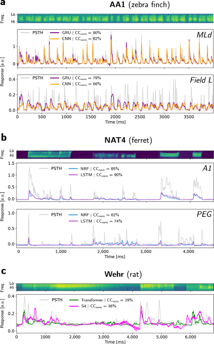
To characterize the ability of models to capture responses in the auditory cortex, we fitted them in a supervised manner on a wide gamut of natural audio stimulus-response datasets. These datasets were collected in different species (ferret, rat, zebra finch) and brain areas (MGB, AAF, A1, PEG, MLd, Field L), under varying behavioral conditions (awake, anesthetized) and using different recording modalities (spikes, membrane potentials). All of them are freely accessible on online repositories and were used with respect to their original license. Because the “NS1“²², “NAT4“^31,78, and “Wehr“^24,44 datasets have already been used in a previous study from our group and their pre-processing pipelines have been extensively described in the associated article²⁷, we only describe here the new datasets added to the current study. The corresponding data pre-processing methods are representative of what was performed in the previous datasets.

AA1 datasets: MLd, field L (zebra finch)

These two datasets consist in single-unit responses recorded from two auditory areas (MLd and Field L) in anesthetized male zebra finches, by Frederic Theunissen’s group at UC Berkeley^43,46,79. Stimuli were composed of short clips (<5 s) of conspecific songs to which animals had no prior exposure, and were modeled by log-compressed mel spectrograms with 32 frequencies ranging 0–16 kHz, at a temporal resolution of 1 ms. Extracellular recordings yielded a total of 50 single units in each area after spike sorting. Spike trains were binned in non-overlapping windows of 1 or 5 ms, matching the resolution of the stimulus spectrogram. Sounds were presented with an average of 10 trials, and the PSTHs were obtained for each neuron and stimulus after averaging spike trains across trials and smoothing with a 21 ms Hanning window^26,80. For each neuron, recordings were performed in response to the same 20 audio stimuli, thereby allowing the training of a single model to predict the simultaneous activity of the whole population (i.e., a “population coding” paradigm).

These data, also referred to as “AA1“, are freely accessible from the CRCNS website (https://crcns.org/data-sets/aa/aa-1/about) and were used with respect to their original license.

Asari dataset: A1, MGB (rat)

This dataset consists in single-unit responses recorded from primary auditory cortex (A1) and medial geniculate body (MGB) neurons in anesthetized rats, by Anthony Zador’s group at Cold Spring Harbor Laboratory^11,44. Stimuli were natural sounds typically lasting around 2–7 s, and originally sampled at 44.1 kHz and then resampled at 97 kHz for presentation. Their associated cochleagrams were obtained using a short-term Fourier transform with 54 logarithmically distributed spectral bands from 0.1 to 45 kHz, whose outputs were subsequently passed through a logarithmic compressive activation. The temporal resolution of stimulus cochleagrams and responses was set to 5 ms. Because for each cell, recordings were performed in response to a different set of probe sounds, we could not apply the population coding paradigm, and one full model was fitted on the stimulus-response pairs for each unit. Contrary to the other datasets, recordings here are intracellular membrane potentials obtained through whole-cell patch-clamp techniques. One remarkable feature of these data is their very high trial-to-trial response reliability, making the noise-corrected normalized correlation coefficients of model predictions almost equal to the raw correlation coefficients (see “Performance metrics” subsection).

Despite the good signal-to-noise ratio of this dataset, some trials are subject to recording artifacts and notably to drifts, which may be caused by motion of the animal and/or of the recording electrode, or electromagnetic interferences with nearby devices. Note that drifts do not contaminate supra-threshold signals resulting from spike-sorted activity, such as PSTHs, because they are strictly positive and thus have a guaranteed stationarity. In order to remove these drifts, we detrended all responses using a custom approach further explicited in Supplementary section “Detrending with MedGauss filter”.

Similar to the previous dataset, these data can be found on CRCNS website (https://crcns.org/data-sets/ac/ac-1) as a subset of the “AC1” dataset.

Neural response fitting task

Because the current benchmark directly builds upon a previous study conducted by our group²⁷, performances and model trainings were conducted according to the same methods, which we describe again below.

Task definition

Neural response fitting is a sequence-to-sequence, time series regression task, taking a spectrogram representation (xin {{mathbb{R}}}^{Ftimes T}) of a sound stimulus as an input, and outputting several 1d time series of neural response (one for each unit), (hat{r}in {{mathbb{R}}}^{Ntimes T}). As the latter, we use the Peri-Stimulus Time Histogram (PSTH), which is the average recorded neural response across repeats. The loss function is the mean squared error (MSE) between the predicted time series and the recorded PSTH, and was evaluated for each time bin of each sequence:

where ({hat{r}}_{n}[t]) is the predicted neural response for neuron n at time-step t, r_n[t] the corresponding PSTH, N is the total number of recorded neurons to fit, and T is the total number of time-steps in the time series (to simplify the notations, we drop the time dependencies symbols [t] thereafter).

Performance metrics

The neural response fitting accuracy of the different models is estimated using the raw correlation coefficient (Pearsons’ r), noted CC_raw, between the model’s predicted activity (hat{r}) and the ground-truth PSTH r, which is the response averaged over all M trials r^(m):

where the covariance and variance are computed along the temporal dimension. Assuming neural variability is purely noise and given a limited number of stimulus presentations, perfect fits (i.e., CC_raw = 1) are impossible to get in practice. In order to give an estimation of the best reachable performance given neuronal and experimental trial-to-trial variability, we use here the normalized correlation coefficient CC_norm, as defined in refs. ^80[,81. For a given optimization set (e.g., train, validation or test) composed of multiple clips of stimulus-response pairs, we first create a long sequence by temporally concatenating all clips together. We then evaluate the signal power SP in the recorded responses as:

which allows to compute the normalized correlation coefficient:

When only one trial is available, we set CC_raw = CC_norm, which corresponds to a fully repeatable recording uncontaminated by noise, thereby preventing any overestimation of performances by setting a lower bound in the absence of data.

Optimization process/model training

All models were randomly initialized using default PyTorch methods and trained using gradient descent and backpropagation. Time recurrent models (DNet and StateNets) were trained using BPTT. Each training sample was a full stimulus-response pair whose duration varied between datasets because of the different recording protocols, but also within some datasets (AA1, Wehr, Asari) in order to maximize the amount of trial information for evaluation. We used AdamW optimizer⁸² and its default PyTorch hyperparameters (β₁ = 0.9, β₂ = 0.999). We used a batch size of 1 for all datasets except NAT4, which have a limited number of training examples, and a batch size of 16 for both NAT4 datasets, which have consequently more (see “Supplementary Note 6: Dataset and model details”). The learning rate was held constant during training and set to a value of 10⁻³. We found empirically that these values led to better results.

We split each dataset into a training, a validation, and a test subset, respecting a 70–10–20% ratio as much as possible, depending on the number of stimulus-response pairs available for each cell in each dataset. After each training epoch, models were evaluated on the validation set, and if the validation loss had decreased with respect to the previous best model, the new model was saved. Models were trained until there was no improvement during 50 consecutive epochs on the validation set, at which point learning was stopped, the last best-performing model was saved, and evaluated on the test set. This procedure was repeated 10 times, each corresponding to a random seed, for different train-valid-test data splits and model parameters initializations, and the test metrics were averaged across splits. All models going through the exact same training pipeline (i.e., waveform-to spectrogram transform, training hyperparameters, etc.) ensured fair comparison between them, implying that architectures with higher test accuracy are genuinely better, despite potential differences with their original studies.

Truncated backpropagation through time

With regular BPTT, the entire RNN model is unrolled back in time, creating a graph that grows in size linearly with the sequence length. In addition, for most tasks, old time steps are less informative of the present than the most recent ones, and gradients can either vanish or explode (i.e., “vanishing/exploding gradient problem”)⁷⁵. TBPTT is a variation of this training algorithm aiming to alleviate these computational constraints⁸³. Its principle relies on removing from the graph time steps older than a fixed temporal horizon K₂. If the loss is evaluated every other K₁ time steps, we note this algorithm TBPTT(K₁, K₂). Fig. 8. illustrates the underlying computations. In this study, in order to maximize the number of samples used for training, the loss is evaluated and backpropagated every time step, and therefore K₁ = 1. As a result, we simplify notations by referring to K₂ as K. For the first t < K₂ time steps, the graph is built from the start of the sequence. For generality, the regular BPTT algorithm used to train our models in the main experiments corresponds to TBPTT(K₁ = 1, K₂ = T), T being the sequence length. We also distinguish two sub-cases of TBPTT:

• TBPTT with warmup. The model is initialized with the default (null) hidden state h₀  = 0 at the very start of the sequence (see Fig. 8a). Inputs are then processed sequentially without building the computational graph, up to the K last time steps before loss evaluation. We qualify these first steps as a “warmup”. As a result, the graph starts with a model in an intermediary, non-default, and ecological hidden state resulting from this procedure.

• TBPTT without warmup. Here, warmup steps are skipped and the model is directly initialized to the default hidden state at the Kth time step before loss evaluation (see Fig. 8b). Therefore, the model here does not have access to any prior information at all, making it a fairer comparison to the training of stateless models.

Model interpretability with feature visualization: gradient maps and deep dreams

We propose here a gradient-based iterative method which, for each unit of a trained neural network ({{{mathcal{M}}}}), extracts its nonlinear receptive fields and estimates the auditory features x_i that maximize its responses. This method builds on feature visualization techniques originally introduced in the AI community^38,39,40 and is known as gradient ascent, leveraging the fact that all the mathematical operations in our models are differentiable. The different steps of this approach are illustrated on Fig. 3a and can be summarized as follows:

1. 1.

   As the first input to the model, use the null stimulus ({x}_{0}in {{mathbb{R}}}^{Ftimes T}), a uniform spectrogram of constant value (0 in our case). This initial stimulus is unbiased and bears no spectro-temporal information. From an information-theoretic perspective, it has no entropy. For a parallel with electrophysiology experiments, it is worth noting that the spectrogram of white noise is theoretically uniform too. The absence of spectro-temporal correlations within probe stimuli (which we respect here) is a strong theoretical requirement that led to the use of white noise in the initial development of the linear STRF theory¹⁷, while further studies preferring natural stimuli used advanced techniques to correct their structure¹⁸.

2. 2.

   Pass x₀ through the model and compute its outputs (i.e., the predicted time-series of activation for the whole neural population): (hat{r}={{{mathcal{M}}}}({x}_{0})in {{mathbb{R}}}^{Ntimes T})

3. 3.

   Define a loss ({{{mathcal{L}}}}:{{mathbb{R}}}^{Ntimes T}mapsto {mathbb{R}}) to minimize and compute it from the model prediction (hat{r}). In this paper, we only targeted a single unit n and used the opposite of its activation at the last (Tth) time-step: ({{{mathcal{L}}}}(hat{r})=-{hat{r}}_{n}[T]). To compute the STRF associated with any neural population ({{{mathcal{N}}}}), the following general loss can be used: ({{{mathcal{L}}}}(hat{r})=-frac{1}{{{Card}(N)}}{sum}_{nin {{{mathcal{N}}}}}{hat{r}}_{n}[T]). The choice of this loss function permits to make the connection with the Spike-Triggered Average (STA) approach used by electrophysiologists, and where the stimulus instances preceding the discharge of the target unit are averaged^17,41,42. Models in our study were fitted to PSTHs or membrane potentials and thus output floating point values, which can be viewed as a spike probability. Trying to maximize this value at the present time-step (the last of the time series) by constructing previous stimulus time steps closely mimics STA. Maximizing the average firing rate across the whole stimulus presentation could be interesting to investigate in future studies.

4. 4.

   Back-propagate through the network the gradients of this loss ({g}_{0}=frac{partial {{{mathcal{L}}}}}{partial {x}_{0}}), thereafter referred to as GradMaps. From their definition, these GradMaps can be directly related to linear STRF (see Supplementary text “Bridging the gap between STRFs, gradMaps and dreams: theoretical framework”).

5. 5.

   Use these gradients to perform a gradient ascent step and modify the input stimulus. For simplification, we denote this operation as x₁ = x₀ − αg₀, but some optimizers have momentum and more elaborate update rules. This is notably the case of Adam and AdamW⁸², which were used in our study. We did not use the SGD optimizer as it converged to much higher loss values—so less optimal—in preliminary experiments.

6. 6.

   Repeat these steps until an early stopping criterion is satisfied, in our case after a fixed number of iterations (1500, a value which led to sufficient loss decreases, see curves in Fig. 3). The result of this process is an optimized input spectrogram d = x_i that maximizes the activation of the target unit(s), thereafter referred to as Dream. If we define ({{{mathcal{F}}}}:{{mathbb{R}}}^{Ftimes T}mapsto {{mathbb{R}}}^{Ftimes T}) as one iteration of the above process, such that ({x}_{i}={{{mathcal{F}}}}({x}_{i-1}| {{{mathcal{M}}}},{{{mathcal{L}}}},n)) then recursively get ({x}_{i}={{{mathcal{F}}}}circ {{{mathcal{F}}}}circ cdots circ {{{mathcal{F}}}}({x}_{0}| {{{mathcal{M}}}},{{{mathcal{L}}}},n)={{{{mathcal{F}}}}}^{i}({x}_{0}| {{{mathcal{M}}}},{{{mathcal{L}}}},n)).

This approach does not assume any requirement on the model to interpret. It can produce infinitely long GradMaps, which are relatable to linear STRFs and can be implemented on any architecture, including RNNs like StateNet, but also stateless and transformers.

Dream and GradMap energy

A trace of temporal integration for a model can be simply defined from its GradMap g as the mean over all frequency bands f of squared elements for each latency t. We designate this measure the “Energy” of the GradMap:

GradMap similarity matrix

As shown in the corresponding results section, this matrix aims to identify functional clusters of models based on their GradMaps; it is built using the following methodology.

The GradMaps of the models to compare are first computed with a number of time steps T slightly above their theoretical TRF size. In the case of the present study, stateless models had a TRF size of up to 43 time steps. Therefore, we computed GradMaps of T = 50 time steps for all models, including StateNet. The length of the GradMap should not be much greater than the theoretical TRF size of stateless models; otherwise, correlations between the GradMaps of the latter would artificially tend towards 1, as time steps beyond the receptive field do not receive any gradient and remain unaffected and at their initial value of 0. This step yields one GradMap per neuron, dataset, and model. After a flattening operation into a F × T vector, we compute Pearson’s correlation coefficient as a pixel-wise metric to compare how similar GradMaps are between models, for a given neuron and dataset. The choice of the CC here instead of other distance metrics (e.g., Euclidean) is motivated by the fact that we are comparing the overall structure of the GradMap/STRF (e.g., how inhibitory and excitatory regions are placed relative to each other) rather than its value. Furthermore, the goodness-of-fit of the Linear STRF model, to which we relate the GradMap, is insensitive to changes in scaling and shifting, precisely because the primary evaluation metric in the neural response modeling community is based on the CC too. As a result, if two models present the same GradMap up to an affine transformation, their functional similarity should be classified as perfect, which would not be the case with metrics, such as a pixel-wise MSE.

Statistics and reproducibility

One major contribution of this work is the sheer amount of implemented models and compiled datasets. All models were implemented and trained using PyTorch, a gold-standard library for deep learning in Python, leveraging autodiff. Datasets were pre-processed under the same format of a PyTorch Dataset class for convenience. Jobs required less than 2 GiB and were executed on Nvidia Titan V GPUs, taking tens of minutes to several hours, depending on the complexity of the model. As an example, the population training (5 seeds) of the StateNet GRU model trained in population coding on all 73 NS1 neurons in parallel typically takes less than 10 min. Conversely, the single unit training (5 seeds) of the same model on the 21 neurons of the Wehr dataset takes more than 3 h.

Reporting summary

Further information on research design is available in the Nature Portfolio Reporting Summary linked to this article.