
Often referred to as “liquid gold,” breast milk supports not only for children’s physical health but also for their emotional well-being. It has been linked to greater protection against infections, a lower risk of overweight and type 2…
Blog
-

financial conditions and credit dynamics
Welcome address by Philip R. Lane, Member of the Executive Board of the ECB, at the 5th WE_ARE_IN Macroeconomics and Finance Conference 2025
Frankfurt am Main, 21 October 2025
It is an honour to participate in the fifth edition of the WE_ARE_IN Macroeconomics and Finance Conference and I congratulate the organising committee for putting together an excellent programme.
Let me start this speech by outlining how the ECB makes monetary policy decisions.[1] As expressed in our monetary policy statement:[2]
The Governing Council is determined to ensure that inflation stabilises at its 2% target in the medium term. It will follow a data-dependent and meeting-by-meeting approach to determining the appropriate monetary policy stance. In particular, the Governing Council’s interest rate decisions will be based on its assessment of the inflation outlook and the risks surrounding it, in light of the incoming economic and financial data, as well as the dynamics of underlying inflation and the strength of monetary policy transmission. The Governing Council is not pre-committing to a particular rate path.
My aim today is to review one dimension of this multi-pronged assessment: how we assess the strength of monetary policy transmission. In what follows, I describe some of the analysis that has underpinned this assessment in recent monetary policy meetings.
I will begin by outlining the contribution of monetary policy to financial conditions before reviewing aggregate credit dynamics. Next, I will move to three key factors in determining monetary transmission: first, heterogeneity across member countries; second, the implications of a high level of uncertainty for monetary transmission; and third, the transmission impact of external factors, namely trade tensions and the exchange rate.
Between July 2022 and September 2023, the ECB raised interest rates from -50 basis points to 400 basis points.[3] After a nine-month holding phase, the monetary policy easing cycle started in June 2024. Between then and June 2025, we lowered our policy rates by a cumulative 200 basis points. Since June, our policy rates have remained unchanged.
In capturing the impact of changes in policy rates on the wider financial environment, it is useful to assess blended measures such as financial conditions indices (FCIs), which synthesise the information from a variety of financial asset prices. As such, FCIs extend the concept of the monetary policy stance to a wider set of financial markets and beyond the level of accommodation or restrictiveness that is under the central bank’s direct control. Akin to a stance measure, loose or tight financial conditions tend to stimulate or dampen economic activity, thus representing an upside or downside force acting on inflation.
Typically, FCIs combine – in a static manner that does not allow for feedback from the economy – a broad set of financial variables, including risk-free rates, sovereign and corporate spreads, equity valuations and exchange rates. It is a standard part of our assessment to study a range of FCI measures, including those developed at the ECB, international policy organisations and private-sector versions. Today, I will focus on a new addition to the family of FCI measures: a new “Macro-Finance” FCI that has been developed by ECB staff in order to overcome the “lack of feedback” problem. [4]
The new methodology incorporates mutual feedback between macroeconomic and financial dynamics, such that the Macro-Financial FCI reflects the joint dynamics of macroeconomic variables and financial conditions. As can be seen from the left panel of Chart 1, the overnight rate (€STR), which is closely tied to our policy rates, typically comoves with and sets the direction of the overall index. But there are also several phases in which financial conditions have moved even when the policy rate was stable (Chart 1, left panel).
The decomposition (Chart 1, middle panel) illustrates that, at the onset of the global financial crisis in 2008, plummeting risk asset prices (dark green area) turned from being a stimulative influence on the FCI to acting as a sudden and sharply tightening factor. The widening of sovereign bond spreads during the European debt crisis (light blue area) also provided extra restriction in the years around 2012. During the episode when policy rates were close to their lower bound, compressed long-term nominal rates and negative real interest rates were important sources of accommodation. As a result, the Macro-Finance FCI reached historically supportive levels in late 2021. It then climbed rapidly in the run-up to the first interest rate hike in July 2022, since the term structure of interest rates sequentially moved higher well ahead and in anticipation of our rate hikes and quantitative tightening.
Chart 1
A new “Macro-Finance Financial Conditions Index”
(percentages)
Source: Bletzinger T., Martorana, G. and Mistak, J. (forthcoming).
Notes: The left panel plots the Macro-Finance FCI alongside the €STR. The middle panel shows the index and its decomposition, with contributions estimated in a macro-finance model (Bletzinger, T. et al., forthcoming). The “Short rate” refers to the €STR, the “Long rate” to the ten-year nominal OIS rate, “Real rates” to the one-year real OIS rate in one year’s time and the five-year real OIS rate, “Sov. spreads” to the two- and ten-year euro area GDP-weighted sovereign bond spreads over OIS rates, “Risk assets” to investment-grade corporate bond spreads and the CAPE ratio, and “Euro fx” to the NEER of the euro. The right panel compares the joint fit of euro area HICP inflation and the composite PMI when substituting the index with other measures in the model. The fit of the Macro-Finance FCI is normalised to 100, and the fit of the other models is expressed relative to that benchmark. The Goldman Sachs FCI refers to Stehn et al. (2019) and the weighted average FCI to Arrigoni et al. (2020). The principal component is the statistical factor that explains most of the variation among the financial market variables entering the Macro-Finance FCI.
The latest observations are for 17 October 2025.
In recent years, the Macro-Finance FCI peaked around the end of the 2022–23 monetary tightening cycle. The increase in the index during this period was primarily driven by rising risk-free rates, with adjustments in risk assets playing a more limited role. Since the peak of the tightening cycle, the index has indicated that financial conditions have become noticeably less restrictive, supported by lower short-term interest rates and higher valuations for risk assets, although this has been partly offset by a stronger euro.
Despite this easing, the level of the Macro-Finance FCI remains well above its historical sample average. In part, this can be attributed to a permanent component to the 2022 shift in the monetary policy stance: the re-anchoring of inflation expectations at the two per cent target means that markets do not expect a return to the “low for long” rate environment that had been expected before the pandemic to continue on an open-ended basis.
The new index outperforms other measures when it comes to describing the macroeconomic dynamics of the euro area (Chart 1, right panel). In this regard, it is key to understand that the financial prices and yields that are aggregated into the Macro-Finance FCI influence bank loan dynamics and loan pricing: this summary statistic of (mostly market-based) financial conditions can be interpreted as an important determinant of broader funding conditions, including those set by the banks, which can be collectively labelled as “financing conditions”. In the next section, we turn to a review of credit dynamics.
Lending rates have been declining broadly in line with historical regularities (Chart 2). But there is a detectable difference between developments in the lending rates to households and to firms: the relatively muted decrease in long-term market rates has contained the decline in the cost of household loans, which tend to be priced off the longer end of the term structure of interest rates and have longer fixed-rate periods, relative to loans to enterprises. As outlined above, this is consistent with a permanent component in the 2022 upward shift in policy rates, with no return expected to the “low for long” zone.
Chart 2
Lending rates across hiking and easing cycles
(percentages per annum, series normalised at 0 in t, where t corresponds to the beginning of the policy hike)
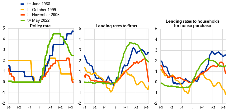
Sources: ECB (MIR) and ECB calculations.
Notes: The ECB relevant policy rate is the lombard rate up to December 1998, the MRO up to May 2014 and the DFR thereafter. The chart reports differences with respect to June 1988, October 1999, November 2005, May 2022 in each of the two panels. Dates are selected as the first change in policy rates in a hiking cycle.
The latest observations are for August 2025.
In terms of credit volumes, household borrowing, primarily for home purchases, has increased steadily. According to the bank lending survey (BLS), the recovery in mortgage demand is supported by improved housing market prospects and lower interest rates (Chart 3, panel A). Corporate borrowing is also gradually recovering, though BLS responses suggest that corporate demand for credit remains subdued, also reflecting global uncertainty and trade tensions.[5]
This evidence raises the question of how credit is evolving compared to past regularities, given macroeconomic conditions and considering the current phase of the policy cycle. The strength of credit dynamics relative to the broader economy can be gauged through a credit-to-GDP gap analysis, which captures the deviation of the credit-to-GDP ratio from historical benchmarks.[6] This gap can be estimated using a range of methodologies, from simple univariate approaches to more sophisticated models that account for the broader state of the economy. Regardless of the method, the gap remains in negative territory (Chart 3, panel B). This may reflect both structural factors and cyclical conditions. However, using multivariate models to control for prevailing cyclical conditions does not change the inference: credit seems to be weak if assessed against past regularities.[7]
A number of structural shifts have been cited to explain a diminished role of credit in advanced economies. For example, households spend less on durable goods and more on services, for which they do not typically need to borrow. Demographic trends can reinforce these trends and explain why mortgages might be in lower demand than in the past. Also, spending on intangible assets – including intellectual property, software and code – has surpassed tangible investments as a share of GDP in major economies since the global financial crisis. And intangibles tend to be financed using internal funds or equity, being harder to pledge as collateral for loans. Even the AI-related investment boom in physical infrastructure, including data centres, has been primarily financed by equity.
But such structural shifts matter less for the euro area than for other economies, which leaves the effects of the previous tightening cycle as an important candidate explanation for the persistent weakness in credit that we observe today.[8] That is, the current credit dynamics most likely reflect the cross-currents arising from the recent easing overlapping with the delayed effects of the past tightening, together with the fact that there is a permanent component to the rate tightening compared to the pre-pandemic levels. For instance, lending rates on new loans are still above those on outstanding loans, and BLS indicators show that the cumulative tightening has not yet been fully reversed.
Chart 3
Credit dynamics
Changes in demand for loans to firms and households
Credit-to-GDP gap across univariate filters and multivariate model-based approaches
(net percentages of banks reporting an increase in demand)
(percentages of GDP)
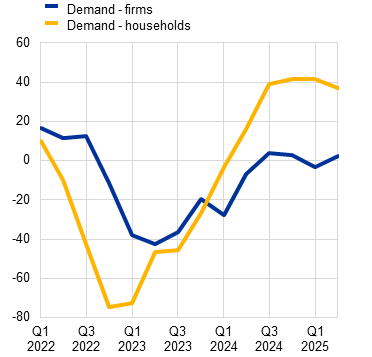
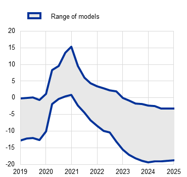
Sources: Left panel: ECB (Bank Lending Survey). Right panel: BIS, ECB and ECB calculations.
Notes: Left panel: the indicators report net percentages for the questions on demand for loans, defined as the difference between the sum of the percentages of banks responding “increased considerably” and “increased somewhat” and the sum of the percentages of banks responding “decreased somewhat” and “decreased considerably”. The indicator for households refers to loans for house purchases. Right panel: the shaded area reports the range of gap estimates across an ensemble of methods and definitions of total credit, using univariate filtering techniques and multivariate models.
The latest observations are the second quarter of 2025 (July 2025 BLS) for the left panel and the first quarter of 2025 for the right panel.
A range of other factors that are not unrelated to the cycle may also help explain why the credit gap indicators remain negative. Heightened risk perceptions and higher bank funding costs, combined with declining excess liquidity, have played a role. In addition, pressures from supervisory and regulatory requirements to maintain solid balance sheets amid rising uncertainties, alongside the goal of supporting financial stability, have kept credit standards tight through the cycle, even as monetary policy has been eased in recent quarters. At the same time, financing from non-bank lenders has remained contained since the start of the monetary policy tightening, despite their secular increasing role in funding the real economy.
Looking in more detail at the sources of external financing for firms other than borrowing from banks, corporate bond issuance has benefited from foreign inflows into euro area bond funds in recent quarters, amid a shift in investor cross-border funds in favour of the euro area. Non-listed equities have also increased recently, likely reflecting activities of private equity funds. One segment of non-bank financing that has been growing significantly in recent years is private credit. Private credit generally refers to non-bank corporate credit provided through bilateral agreements or small “club deals” involving lenders outside the realm of securities investors or commercial banks. Despite a clear expansion in the euro area over recent years, the lion’s share of private credit is originated in the United States.[9] Although numbers vary depending on the exact definition of private credit and source, the size of private credit in the United States is well above €1 trillion, while for the euro area numbers range from around €100 billion to around €300 billion.[10] Taken together, non-bank financing has not grown enough to counteract the weakness in bank lending. The dynamics of all the sources of external finance for euro area firms, including equity financing, but also trade credit and non-bank financing, remain contained by historical standards (Chart 4), hence overall measures of the credit gap, as shown in Chart 3, remain negative.
On net, the ongoing transmission of monetary policy easing to credit volumes has been more gradual than anticipated building on past regularities. Equally unusual has been the pronounced heterogeneity across sectors and across borrower characteristics, which I will discuss next.
Chart 4
Firms’ external financing over time
(annual percentage change and percentage point contributions)
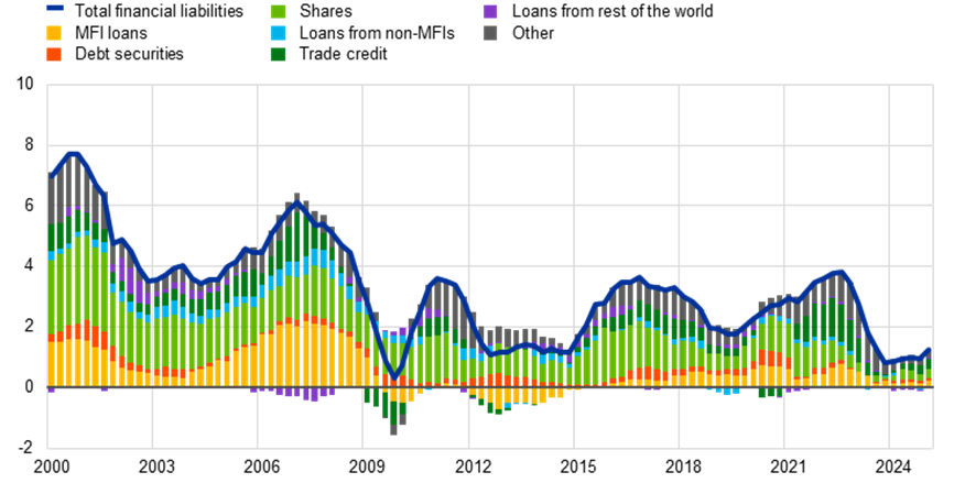
Sources: ECB (QSA, BSI, FVC), Eurostat and ECB calculations.
Notes: MFI loans are corrected for cash polling, loan sales and securitisation. Loans from non-MFIs are corrected for securitisation and they comprise loans from insurance corporations and pension funds (ICPFs) and other financial intermediaries (OFIs). “Other” is the difference between the total and the instruments singled out in the chart; it includes loans from general government, inter-company loans, financial derivatives (net) and other accounts payable other than trade credits.
The latest observations are for the first quarter of 2025.
Heterogeneity in the transmission of monetary policy can affect its overall macroeconomic impact. Differences in sectoral balance sheets and sectoral exposures to macroeconomic shocks can influence the responses of households, firms and banks to changes in financing conditions.[11]
For instance, the growth rate of loans to the manufacturing sector, although recently supported by the surge in activity due to frontloading of euro area shipments to the United States, has been weaker than that of loans to the services sector (Chart 5, Panel A).[12] As manufacturing is capital-intensive, this development connects to the anaemic growth in investment in recent years. Moreover, manufacturing is also working-capital intensive, and therefore especially affected by the cost channel of monetary policy. That a stronger recovery in the manufacturing sector has so far not materialised helps explain a weaker pass‑through of monetary easing via the cost channel than would normally be expected. The underlying reasons could be related to the greater exposure of manufacturing to the external environment, a topic that I will get back to later. By contrast, credit dynamics in the services sector have been driven largely by real estate and leasing activities, supported by recovering domestic demand for housing and durable goods in the euro area.
Chart 5
Heterogeneous credit dynamics across sectors and type of firm
Loans to firms by sector
Lending by firm size and riskiness
(left panel: index = 0 for January 2024, right panel: percentages per annum)
(left panel: index = 0 for January 2024, right panel: annual percentage changes)
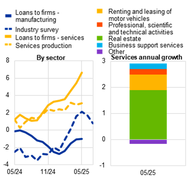
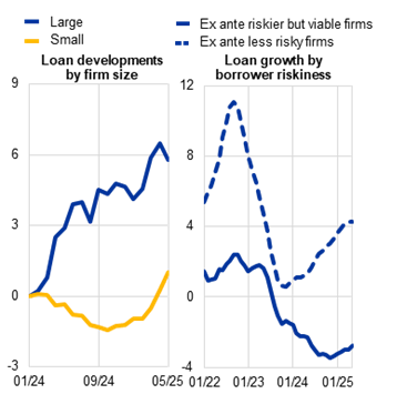
Sources: ECB (ECS, RIAD, BSI, AnaCredit) and ECB calculations.
Notes: Left panel: in the left-hand side chart, the super-sectors are identified from the following NACE sectors: Manufacturing (C), Services (G, H, I, J, L, M, N O, P, Q, R, S, T, U). The industry survey is sourced from ECS and represents the production trend observed in recent three months, while the services production is sourced from STS. The series for the loans to firms in the manufacturing sector and for the industry survey have been smoothed using a three-month moving average. The right-hand side chart represents the growth contribution of selected sectors for April 2025. Right panel: the left-hand side chart represents the index (January 2024 = 0) of the stock of loans by size. Company sizes are defined as small for 50 employees or less, medium for 51 to 250 employees, and large above 250 employees. In the right-hand side chart, loan growth by PD group has been rescaled to match BSI aggregates and purged from PD migrations. High (resp. low) risk firms are those with a PD above (resp. below) 1.6%, the third quartile of PD in lending flows.
The latest observations are for May 2025 for AnaCredit, July 2025 for ECS.
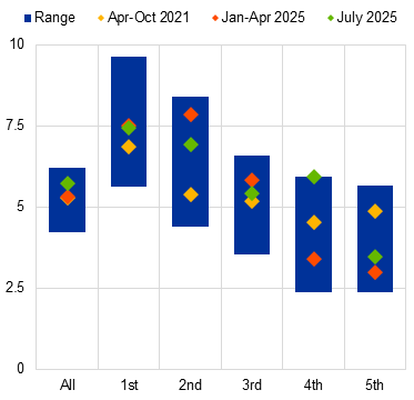
At the firm level, credit growth is increasingly concentrated among larger and less risky firms (Chart 5, panel B). Results from the survey on the access to finance of enterprises (SAFE) confirm that small firms have experienced a more muted decline in external financing costs than larger producers. This points to contained transmission via the balance sheet channel and the risk-taking channel of monetary policy. Smaller firms, being more vulnerable to current macroeconomic risks, have therefore suffered sharper balance sheet losses. At the same time, banks have been more reluctant to extend credit to riskier borrowers.[13] Since small firms also face greater obstacles in accessing alternative sources of funding, banks’ reluctance to lend further tightens the financial constraints facing smaller and riskier firms and weighs on their ability to invest.[14]
Chart 6
Heterogeneous monetary policy pass-through in mortgage and housing markets
Growth momentum of bank loans to households by country
Changes in new mortgage applications by households by income quintile
(percentages per annum)
(percentage points)
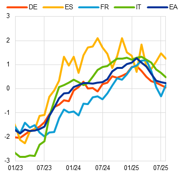
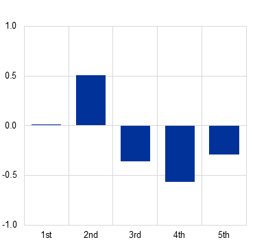
Sources: ECB (BSI, CES) and ECB calculations.
Notes: Left panel: momentum is defined by the difference between the (3m-o-3m annualised) and the annual growth rate. Right panel: The chart reports the percentage point change in the share of households that applied for mortgages relative to before the monetary policy tightening, broken down by income quintile. Income quintiles are computed over the weighted distributions of the variable at the country level and by wave.
The latest observations are for August 2025 for the left panel and July 2025 for the right panel.
Household loan dynamics have also shown dispersion across countries, highlighting the role of both the collateral and cash-flow channels in monetary transmission during the tightening and easing phases of the cycle (Chart 6, panel A). Differences in national mortgage markets are a key factor, reflecting institutional features such as the share of adjustable-rate mortgages (ARMs) and their maturities.[15] Historical regularities show that the pass-through is stronger in mortgage markets with a higher share of adjustable-rate mortgages and shorter maturities, reflecting both the larger movements in short-term compared to long-term market rates and the faster repricing of the total stock of outstanding loans when fixation periods are shorter.[16] Indeed, over the past two decades, floating-rate mortgages — which are more reactive to the policy rates – have become less popular in the major euro area economies. The shift in the types of mortgages means monetary policy takes longer to work its way into households’ debt payments. This delay in transmission means that, despite recent rate cuts, average mortgage rates are expected to rise further and drag on consumption for a number of years to come as households remortgage on to higher rates after completing long-term fixed deals.[17] Moreover, through the collateral channel, recent interest rate cuts have pushed up asset values more in countries with high ARM shares, thereby boosting collateral values.
After a period of declining mortgage applications during the tightening period, mortgage applications have started to increase in recent quarters. Higher income households, however, have maintained lower mortgage applications compared to the pre-tightening period (Chart 6, panel B). Instead, mortgage application growth has come mostly from lower-income households, possibly reflecting the need to maintain consumption or housing purchase plans in spite of declining real wages and with less savings, especially if they spend a large share of their income on basic goods. Thus, we see a shift in the composition of mortgage demand.[18]
Summing up, the change in borrower composition and the muted risk appetite of banks point towards the risk-taking and balance sheet channels of monetary policy operating less strongly for lower-income households and smaller firms during the easing cycle. Since these groups typically have higher marginal propensities to consume and invest, this heterogeneity in transmission may reduce the effectiveness of recent interest rate cuts in stimulating aggregate demand in the current context of high global uncertainty.[19]
An important factor that may distort and at times suppress the transmission of monetary policy is uncertainty. Over the past year, economic policy uncertainty has risen sharply, reaching record levels in April, largely driven by trade tensions and geopolitical risks (Chart 7, left panel). Financial market volatility has, instead, remained subdued (Chart 7, right panel). While uncertainty has eased somewhat in recent months, it remains at historically high levels on both sides of the Atlantic according to newspaper-based measures, close to the peak seen during the COVID-19 pandemic.
Monitoring elevated uncertainty is crucial in analysing credit dynamics for two main reasons.
First, it directly lowers credit demand and credit supply. ECB staff finds that unexpected increases in economic policy uncertainty have a negative effect on bank lending in the euro area.[20] When economic policy uncertainty spikes unexpectedly, households and businesses tend to delay their consumption and investment decisions, as the value of waiting for additional information increases.[21] As a result, the financing needs and loan demand of firms drop in synch, as shown in recent BLS replies. On the lender side, banks may adopt a more cautious stance as well, delaying the approval of new loans and thereby affecting the availability of credit within the economy.[22] These effects are amplified if financial market volatility spikes up.
Second, ECB staff also finds that elevated uncertainty diminishes the impact of monetary policy easing on firms’ investment.[23] Even when a central bank lowers rates to encourage banks to lend and firms and households to borrow, spend and invest, the impact may be weaker or slower during periods of heightened uncertainty.
On its own terms, if uncertainty weakens monetary transmission, this implies that a more powerful monetary intervention is required to deliver a given policy objective. At the same time, monetary policymakers must strike a balance between the incentives to act more powerfully and the incentives to wait and see whether an uncertainty spike self-corrects in a timely manner. [24] As noted in our September monetary policy statement, uncertainty has declined compared to the peaks in the second quarter but remains elevated compared to historical norms.
Chart 7
Measures of uncertainty
(left panel: index, right panel: annualised percentage points)
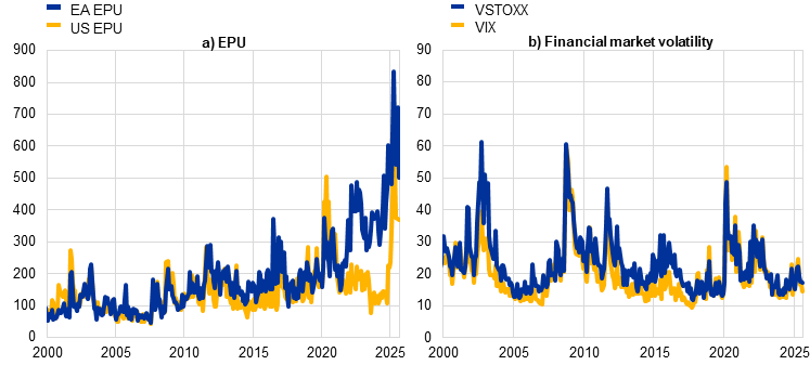
Sources: Baker, Bloom and Davis (2016), Bloomberg and ECB calculations.
Notes: The US EPU and EA EPU are estimated by Baker, Bloom and Davis (2016). The EA EPU is constructed as a GDP weighted average of country-level indices.
The latest observations are for August 2025.
The strength of monetary policy transmission depends on the configuration of the macroeconomic shocks hitting the euro area. Two (interconnected) external shocks are currently shaping euro area macroeconomic dynamics. First, a large portion of the uncertainty highlighted above stems from outside the EU, reflecting unpredictable shifts in foreign economic policies and concerns about the future course of geopolitical tensions. Second, there has been a substantial appreciation of the euro.
The recent tariff agreement between the EU and the United States has eased trade policy uncertainty and overall economic policy uncertainty to some extent, yet important questions remain. A key source of risk is the ongoing tensions in US-China trade relations. If these tensions persist, Chinese exporters would have stronger incentives to redirect shipments toward non‑US markets, heightening competition for European firms.[25] Such increased competition would weigh on demand in export-intensive and import-competing European sectors, reducing corporate earnings and weakening the transmission of monetary easing through the cash flow and balance sheet channels. In addition to these demand-side effects, trade tensions may disrupt supply chains, amplifying the risk faced by banks in lending to firms participating in international trade and thus amplifying conditions of uncertainty.[26]
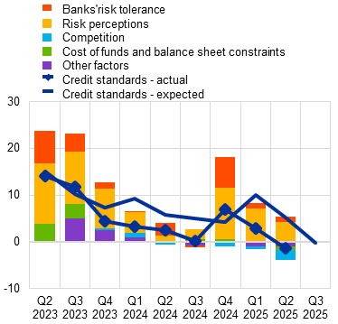
Trade fragmentation is also heightening concerns about elevated risks to economic conditions. According to the BLS, perceived risks related to the economic outlook have been contributing to a tightening of credit standards since the last quarter of 2024 (Chart 8, panel A), despite the fact that policy rates have been reduced for much of this period.
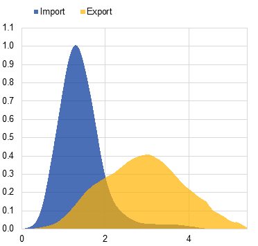
Based on the sector-country allocation of bank credit to firms that trade with the United States, the greater risk lies with loans to exporters. This is due to the higher relative size of these exposures, and to the specifics of the July tariff agreement, which introduced a broad-based US tariff of 15 per cent for EU goods, although with some exceptions and carveouts (Chart 8, panel B).[27] Looking ahead, it is crucial to keep an eye on the asset quality of lenders that have significant exposure to tariffs. While so far there are limited signs of deterioration in asset quality, banks’ perception of lending to firms more affected by tariffs could impair the supply of credit, weakening the monetary policy easing impulse.
Chart 8
Credit standards and US trade exposure: drivers of corporate lending
Changes in credit standards for loans to firms
US trade exposure
(net percentages of banks reporting a tightening of credit standards and contributing factors)
(percentages of gross value added)
Sources: Left panel: ECB (Bank Lending Survey) and ECB calculations; right panel: ECB (AnaCredit), European Commission and ECB calculations.
Notes: Left panel: “Credit standards – actual” are changes that have occurred, while “Credit standards – expected” are changes anticipated by banks. Net percentages are defined as the difference between the sum of the percentages of banks responding “tightened considerably” and “tightened somewhat” and the sum of the percentages of banks responding “eased somewhat” and “eased considerably”. The net percentages for the “other factors” refer to further factors which were mentioned by banks as having contributed to changes in credit standards for loans. Right panel: trade exposure at the sector level is computed as import or export to the US over gross value added by sector. Trade exposure at the bank level is computed as a weighted average using AnaCredit. The chart represents a kernel density of exposures in December 2024.
The latest observations are for the second quarter of 2025 (July 2025 BLS) for the left panel and December 2024 for the right panel.
Households currently benefit from a strong labour market, a low and stable inflation outlook and favourable conditions in the housing markets. However, those working in certain sectors, in particular manufacturing, are increasingly worried about the negative effects of tariffs, expecting income declines and tighter credit access. As a result, they anticipate submitting fewer credit applications (Chart 9, panel A). At the same time, lower-income households are starting to report increasing difficulties in meeting mortgage payments (Chart 9, panel B). Higher financial distress rates of households pose a downside risk for the transmission of the recent interest rate cuts.[28]
Chart 9
The effects of perceived higher tariff exposure for households’ credit market expectations and increasing household financial difficulties.
US tariffs and households’ credit market expectations
Households’ difficulty meeting mortgage payments
(percentage points)
(percentages of respondents)
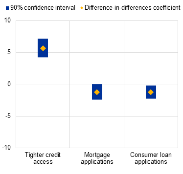
Sources: ECB (CES) and ECB calculations.
Notes: Left panel: the chart shows coefficients from a difference-in-difference regression of expectations of credit market access and applications of households on an indicator for whether the household reported that its financial wellbeing would be negatively affected by US tariffs interacted with a dummy for the period April 2025 to July 2025. Right panel: the chart shows the share of CES respondents reporting difficulties meeting mortgage payments in the past 12 months, by income quintile. Income quintiles are computed over the weighted distribution of the variable at the country level and by wave.
The latest observations are for July 2025.
Turning to the impact of euro appreciation on monetary transmission, there are two broad channels. First, euro appreciation affects credit demand and credit supply through its impact on macroeconomic dynamics. Second, euro appreciation affects the balance sheets and funding conditions of banks.
In relation to the former channel, euro appreciation is typically associated with slower growth and lower inflation over a multi-year horizon. At the same time, the impact varies across euro area corporates, such that it is important to take into account the differences across bank-firm pairs. In one direction, the appreciation of the euro against the US dollar and other currencies lowers price competitiveness for European exporters and import competers. In the other direction, firms that do not have large USD-denominated revenues but pay for intermediate input costs (e.g. energy) in foreign currencies (especially the dollar) benefit from a term-of-trade improvement from euro appreciation.[29]
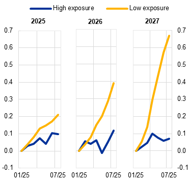
For credit supply, the net impact via the real economy depends on their client mix: institutions more exposed to tradable sectors may face tougher conditions, but banks with a high presence in the non‑tradable economy may benefit from the stronger purchasing power of their customers (Chart 8, panel B). On the one hand, market analysts are already discounting exposures to the United States in their estimates of euro area banks’ profitability prospects (Chart 10, panel A), despite the overall positive expectations for the sector.[30] On the other hand, an appreciation of the euro improves the euro area’s terms of trade by lowering import prices, supporting real incomes and potentially making borrowers’ balance sheets stronger, eventually increasing banks’ willingness to serve customer segments benefiting from cheaper imports.
Turning to the latter channel, the depreciation of the dollar has a direct impact on the effective quantity of USD-denominated liquidity. USD-denominated assets constitute an integral part of the liquidity management practices of banks, both for those with active business lines in the United States and for those that use liquid dollar assets as hedging devices.
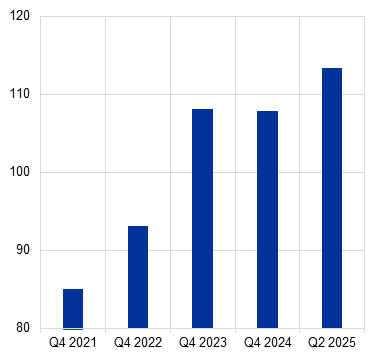
During the tariff turmoil, the unusual combination of a sell-off in US Treasury securities and a weakening dollar made it more difficult for euro area banks to rely on their USD-denominated liquid assets – once considered safe havens offering downside protection – to cushion lending and funding pressures.[31] Banks with lower USD-denominated liquidity buffers saw their bond spreads widen more sharply. While the USD LCR is not mechanically affected by movements in the exchange rate and the liquidity regulation in the EU generally does not require banks to hold LCR levels in foreign currencies above 100 per cent, excessively low levels of USD LCR may become a source of fragility for banks during episodes of large exchange rate volatility.[32] Since the euro area banking system has made progress in increasing their USD LCRs in recent years (Chart 10, panel B), it did not experience sizeable liquidity strains even at the height of the exchange rate volatility in early April, though the episode may have altered the algebra of liquidity management for the remainder of the year.[33]
Since euro appreciation reflects a global portfolio rebalancing that has triggered higher capital inflows into the euro, this may provide a windfall of funding opportunities for euro area banks while also creating the market conditions that have further contributed to the compression of bank bond spreads. Against this backdrop, bank bond issuance activity has rebounded since May, including a pickup in USD-denominated bonds.[34] Moreover, globally active euro area banks, for which USD funding represents a non-negligible share of total liabilities, can pass through the easier funding conditions to other banks via interbank money market lending.[35]
Euro appreciation also generates valuation losses on the asset side of euro area banks but also effective funding cost reductions on the liability side. The repercussions of these two countervailing effects on the intermediation capacity of banks and credit supply depends on the aggregate net exposure but also on whether exposures via assets and liabilities are unevenly distributed in the cross-section.
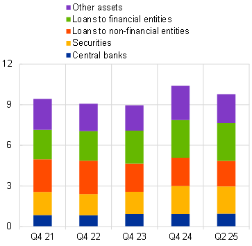
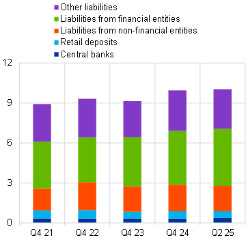
Exposures on the asset side can be sizeable. Total USD exposures represented almost 10 per cent of the assets of the euro area banking system in the second quarter of 2025.[36] Among the banks with USD asset exposures, the interquartile range of the ratio of these exposures over total assets lies between 5 per cent and 25 per cent as at the second quarter of 2025, with around one half of the overall exposures accounted for by loans of banking groups active outside of the euro area (Chart 11, Panel A). In general, the valuation impact is relatively contained when cast against the capital buffers of the euro area banking system or previous episodes of valuation losses associated with, for instance, fluctuations in the value of sovereign holdings.
Moreover, euro area banks also have a substantial part of liabilities denominated in USD, with an interquartile range ranging between 7 per cent and 28 per cent as at the second quarter of 2025, and with a total amount similar to that of assets. A substantial share (43 per cent) of USD-denominated liabilities is provided by financial entities (Chart 11, panel B) and is therefore relatively volatile, especially during market turbulence. Overall, the net exposure in USD is rather stable over time: for banks with USD exposures, it is close to zero for the median bank and slightly negative in the aggregate at -2 per cent of banks’ assets. Moreover, reflecting the asset-liability management practices and the business models of banks with significant USD activity, net exposures are typically relatively unreactive to fluctuations in the exchange rate, policy rates or the business cycle. At the same time, the combined presence of substantial USD-denominated off-balance sheet exposures and volatile funding means that sudden changes in these net exposures cannot be ruled out. An increased probability of such a risk event would then generate pressures on both sides of banks’ balance sheets and potentially downward pressure on on-balance sheet exposures like loans to the real economy.[37] Moreover, the composition of USD liabilities, dominated by funding from financial customers and with a limited share of retail deposits, can exacerbate these pressures by making funding more flight‑prone, thereby increasing vulnerability in a stress scenario.
Chart 10
Earnings outlook in the banking sector and US dollar exposure
Bank ROE forecast revisions by exposure to US exporting borrowers
USD Liquidity Coverage Ratio
(percentage point change relative to January 2025)
(percentage)
Sources: Left panel: LSEG (I/B/E/S) and ECB calculations; Right panel: ECB Supervisory Reporting and ECB calculations.
Notes: Left panel: forecast revisions are calculated at the bank level for each end-year (fixed event), relative to the January 2025 forecast. Median forecast revisions for each group of banks are taken. High exposure banks are those in the upper quartile of exposure to sector-countries with a high share of exports to the US. Right panel: USD Liquidity Coverage Ratio for a balanced sample of banks.
The latest observations are for July 2025 for the left panel and the second quarter of 2025 for the right panel.
Chart 11
USD assets and USD liabilities of euro area banks
Bank assets denominated in USD
Bank liabilities denominated in USD
(percentages of total assets in the banking system)
(percentages of total assets in the banking system)
Sources: Both panels: ECB Supervisory Reporting and ECB calculations.
Notes: Left panel: sum of USD assets, converted to EUR at the current exchange rate on each date, across a balance sample of banks that report in NSFR templates, divided by total assets of a balanced sample of banks that report in FINREP. “Other assets” include loans not classified as “Loans to non-financial entities” or as “Loans to financial entities”, and include derivatives exposures and other residual assets, but not off-balance-sheet items. Right panel: Sum of USD liabilities, converted to EUR at the current exchange rate on each date, across a balanced sample of banks that report in NSFR templates, divided by total assets of a balanced sample of banks that report in FINREP. “Other liabilities” include capital instruments and other residual liabilities, as well as derivatives.
The latest observations are for the second quarter of 2025 for both panels.
My aim in this speech has been to showcase some of the analysis that has underpinned our assessment of the strength of monetary transmission in recent monetary policy meetings. In overall terms, monetary policy transmission is progressing smoothly. Yet, within this overall favourable environment, the analysis reported above highlights that it is also important to take into account significant differences across different types of banks, firms and households, across different sectors and across countries.
More generally, the analysis shows that the strength of monetary transmission is time-varying and also depends on the configuration of domestic and external macroeconomic shocks hitting the euro area economy. Accordingly, it makes sense to maintain a meeting-by-meeting and data-dependent approach to assessing the strength of monetary transmission at any given point in time. In turn, this feeds into our overall monetary policy decision making, alongside our other assessment criteria: the inflation outlook and the risks surrounding it, together with the dynamics of underlying inflation.
Continue Reading
-

Longsys Launches Industry’s First Integrated-packaging mSSD, Enabling Flexible and Efficient Manufacturing
SHENZHEN, China, Oct. 21, 2025 /PRNewswire/ — Longsys (301308.SZ) has unveiled the industry’s first integrated-packaging mSSD (Micro SSD), developed under its “Office is Factory” model. By redefining how SSDs are…
Continue Reading
-

Pair of ‘holy’ islands in eerily green African lake hold centuries-old relics and mummified emperors — Earth from space
QUICK FACTS
Where is it? Dek and Daga, Ethiopia [11.907552854, 37.285011102]
What’s in the photo? A pair of islands in the middle of the green-colored Lake Tana
Who took the photo? An unnamed astronaut onboard the International Space Station
When…
Continue Reading
-

ASUS TUF Gaming Unveils Call of Duty: Black Ops 7 Edition AMD Radeon RX 9070 XT | ASUS Pressroom
About ROG
Republic of Gamers (ROG) is an ASUS sub-brand dedicated to creating the world’s best gaming hardware and software. Formed in 2006, ROG offers a complete line of innovative products known for performance and quality, including…
Continue Reading
-

Artificial intelligence and deep learning in breast cancer detection:
Introduction
Breast cancer remains a global health challenge, with over 2.3 million new cases diagnosed annually, underscoring the need for effective early detection and accurate diagnosis methods.1,2 Traditional screening methods, such as…
Continue Reading
-

‘Schitt’s Creek’ Gets FAST Channel On Canada’s CBC
Schitt’s Creek made the calamitous Rose family famous famous, and their escapades can now be found in one place in Canda.
CBC has added to its FAST streaming portfolio with the launch of a Schitt’s Creek channel,…
Continue Reading
-

Trump vows to reach a ‘fantastic deal’ with China after future meeting with Xi
WASHINGTON — WASHINGTON (AP) — President Donald Trump said Monday that the U.S. commands “great respect” from Beijing and that he will reach a “fantastic deal” with Chinese President Xi Jinping when the two leaders meet soon.
Trump’s…
Continue Reading
-

Researchers discover how a brain circuit allows eating despite anxiety
How do mammals manage to eat in situations that cause anxiety, step into exposed spaces, or slow down when anxiety drives them to keep moving? A new study pinpoints a leptin-sensitive circuit in the lateral hypothalamus that helps…
Continue Reading
-
From Passive to Pleasant: Validation and Application of the Learning E
Introduction
Student enjoyment pertains to the sense of pleasure or satisfaction that students derive from the learning process. Enjoyment of a learning activity fosters sustained motivation, enthusiasm, and positive emotions that enhance the overall learning experience.1,2 This aspect of education is closely intertwined with both student interest and motivation. While these three concepts share connections, they represent distinct dimensions of a student’s engagement with learning. Student interest involves the curiosity and attraction that they feel toward a particular subject or activity, whereas motivation encompasses the factors that drive students to dedicate themselves to the learning process.3 According to the Self-Determination Theory, motivation is enhanced when learners experience autonomy in learning, feeling of competence, and sense of relatedness to other students.4 Similarly, constructivist theory emphasizes that learning is most engaging when students actively construct knowledge through hands-on activities, real-world problem-solving, and collaborative interaction.5 This indicates that motivation is dependent on multiple factors that include the learner’s psychological needs, personal values, and the social context in which learning occurs. The synergy of enjoyment, interest, and motivation is crucial for the academic achievement of students, as these elements significantly influence student engagement with the overall learning experience.2–7 This combination contributes to a positive and effective learning atmosphere, fostering not only academic success but also a genuine passion for knowledge.4,8 While these concepts may overlap, each would play a distinctive role in shaping and enhancing the overall quality of the student’s learning experience.
Given the close relationship between motivation and positive learning experiences, student enjoyment can be seen as a complementary driver of engagement, influenced by factors such as teachers’ proficiency, students’ self-efficacy, and the complexity of the subject matter. This perception drives the ongoing search for more engaging and effective instructional formats, highlighting the need to explore and refine pedagogical strategies that address diverse learning needs. Within this context, lectures remain one of the most scrutinized instructional methods in higher education. Over the past decades, the debate about the effectiveness of didactical lectures has persisted, yielding mixed outcomes that reflect the diverse perspectives among educators and the heterogeneous opinions held by students regarding instructional methods.9–11 Didactic lectures have often faced criticism for their perceived lack of student enjoyment, primarily stemming from their reliance on passive one-way information delivery.12–14 In contrast to active learning methodologies such as problem-based learning (PBL) or team-based learning (TBL), students frequently perceive didactic lectures as boring or ineffective.12–14 In response to these critiques, many educators are adopting a more interactive approach to their lectures. They seek to engage students by incorporating entertaining activities such as real-life scenarios15 games16 technology17 or problem-solving components18 during lectures. However, despite these efforts, there are no universally clear guidelines on how to organize lectures that are not only educational but also enjoyable. Practical tips and useful recommendations published in Medical Teacher offer valuable strategies to help educators transform didactic lectures into interactive, and effective sessions.19
A skilled lecturer possesses the ability to attract the attention of students and enhance their enjoyment through various innovative techniques that include incorporating personal experiences, telling jokes, and sharing relevant stories.2,20 The impact of such engaging teaching strategies extends beyond mere enjoyment; they have the potential to significantly influence the overall motivation and performance of students. An instructor with an entertaining and effective teaching style can successfully convey information, fostering a positive and dynamic learning environment that may surpass the positive ratings of active learning.21 In contrast, some instructors may lack the talent to effectively engage and motivate their students, resulting in a potential adverse effect on the students’ overall academic performance. However, it is worth noting that Deslauriers et al demonstrated that while students may rate enjoyable lectures positively and even feel they learned more compared to active learning sessions, objective measures showed that actual learning was greater in active learning environments that were perceived lower, indicating that high enjoyment does not necessarily lead to better learning.22
The ongoing debate about the effectiveness of teacher-based learning methods (or passive instruction) versus student-based learning methods (or active instruction) is persistent despite the numerous studies conducted over the past decades. The multitude of factors influencing students’ enjoyment in both types of instruction could be responsible for the variable preferences or mixed feelings of enjoyment among students. In addition to the educational environment, factors such as teachers’ varying skills and experiences and the difficulty level of certain subjects all contribute to and impact the level of enjoyment experienced during a teaching activity.1,13,14,22 Since enjoyment influences engagement, the present study aimed to develop and validate an objective instrument for systematically measuring students’ enjoyment in different pedagogical contexts, and to apply it in evaluating the enjoyment of first-year students in Physiology lectures. This kind of tool would help teachers to examine teaching strategies, identify the origins of differences in student enjoyment, and understand how the same strategies will yield different results when used by different teachers or when applied to different contexts. We sought to apply this scale objectively to measure the enjoyment scores of didactic lectures and investigate associated factors. Through this research, we aim to contribute valuable insights into the dynamics of student enjoyment, offering a tool that explores the factors that influence students’ learning experiences.
Methods
Study Design and Participants
In this cross-sectional study, we assessed the enjoyment levels of first-year undergraduate medical and dental students during two physiology lectures. Lectures were delivered by experienced and highly rated professor, followed a didactic format with interactive discussion to encourage student participation and lasted 50 minutes. First-year medical and dental students were chosen to participate in this study because they were newcomers to university health profession education, suggesting that they were unlikely to have developed preferences for specific instructional methods at this early stage. The University Research Ethics Committee granted approval for the study under the reference number “HEC-10-2023/24-F-M.” Informed consent was obtained by first providing students with a briefing sheet detailing the study’s aims and purpose. Students were informed that their participation was entirely voluntary and would not affect their marks or academic evaluation. They were then asked to sign a consent form confirming that they had read and understood the information and agreed to participate in the study. A total of 112 (68%) students participated in the study, with 32 (out of 47) participants from the dental college and 80 (out of 118) from the medical college. The measuring instrument was distributed to all students immediately following the teaching session.
Data Collection Tool
The Learning Enjoyment Scale (LES) was developed by the investigators as a comprehensive and objective measure of students’ enjoyment in the learning process (Figure 1). A brief description of the scale with guidance on its analysis, has been previously published as a data note.23,24 The scale items are strategically based on the major categories of Bloom’s Taxonomy, specifically focusing on cognitive knowledge and affective attitudes. The LES comprises six items: knowledge, comprehension, application, analysis, concentration, and enjoyment. Students are requested to assess each item using a five-point Likert scale, ranging from 1 to 5 (1 = strongly disagree, 2 = disagree, 3 = unsure, 4 = agree, and 5 = strongly agree). The minimum and maximum total scores across the six items are 6 and 30, respectively. If all responses are agree (ie, Likert scale 4), the total score is 24, representing 80% of the maximum score. Conversely, if all responses are unsure (ie, Likert scale 3), the total score is 18, which accounts for 60% of the maximum score. Consequently, an excellent score is deemed to be above 80% (25–30), an acceptable score falls within the range of 60–80% (18–24), and a low score is defined as less than 60% (< 18). These thresholds facilitate clear interpretation of students’ enjoyment levels and are consistent with educational standards for assessing performance and satisfaction in academic settings.
Figure 1 The Learning Enjoyment Scale. The Learning Enjoyment Scale (LES) is a comprehensive tool developed to assess student enjoyment. (A) contains six items measuring perceived learning, confidence, interest, and overall enjoyment. (B) contains six items assessing factors influencing enjoyment, such as teacher talent, content difficulty, participation, achievement of objectives, stress levels, and skill satisfaction.
The second section of the scale (enjoyment attributes) assesses the influence of various factors on students’ enjoyment. These factors include the teacher’s talent, the complexity of the topic, student participation, fulfillment of objectives, perceived stress levels, and the development of skills. The analysis of this section provides detailed understanding of the specific elements that impact students’ enjoyment during the learning process.
Data Analysis Plan
The statistical analysis for this study was carried out using the Statistical Package for Social Sciences (SPSS), version 26. Reliability analysis was applied to determine the internal consistency of the Learning Enjoyment Scale (LES) through Cronbach’s alpha. The obtained value of Cronbach’s alpha was interpreted, with values greater than 0.7 indicating a good level of internal consistency. General tendencies of the Learning Enjoyment Scale items were analyzed using the mean ± SD. The comparisons and associations between LES items or LES attributes and the total score categories were analyzed using the Spearman correlation and the chi-square test with Fisher’s exact correction, as appropriate. A p-value of <0.05 was considered statistically significant.
Results
Table 1 displays the items of the Learning Enjoyment Scale (LES), the learning domain assessed by each item and the general tendency of students to respond to each item. According to the Likert scale analysis, the overall tendency of students’ responses in this study was “agree”. Reliability and validity of the scale were confirmed in this study: internal consistency was excellent, with a Cronbach’s Alpha of 0.91. Exploratory Factor Analysis (EFA) supported the theoretical six-domain structure, with the first two components explaining 80.5% of the variance. Inter-item correlations ranged from 0.57 to 0.81, indicating meaningful relationships between items. These psychometric properties demonstrate that the LES is a robust and valid instrument for measuring students’ enjoyment in learning contexts.

Table 1 General Tendencies of Students’ Responses to the Learning Enjoyment Scale Items
Table 2 shows the relationships of the six items of the LES with the three categories of the total score (Low, Acceptable and Excellent). The table shows a significant relation between the students’ responses and the LES categories, with “agree” being the most frequent response and “acceptable” being the major LES category.

Table 2 Examining Students’ Responses to Learning Enjoyment Scale Questionnaire Items in Relation to Total Score Categories
Table 3 displays the association between enjoyment attributes and the three categories of the total score. Enjoyment of a learning activity was strongly related to teachers’ talent (P< 0.001), difficulty of the topic (P< 0.001), students’ active participation during the activity (P< 0.001), fulfillment of the objectives (P< 0.001), low level of stress during the activity (P< 0.001) and self-perception of acquired skills (P< 0.001).

Table 3 Relationships Between Enjoyment Attributes and Categories According to the Total Learning Enjoyment Scale
Most dental students (97%) and medical students (95%) showed either acceptable or high enjoyment scores for the Physiology lectures. The difference between students in the two colleges was not statistically significant (Table 4).

Table 4 Comparison of the Total Learning Enjoyment Scale Scores of Dental and Medical Students
Table 5 demonstrates moderate to strong positive Spearman correlations (ρ = 0.35–0.57) between the Total LES Score and all enjoyment attributes, indicating that students with higher LES scores consistently reported more favorable perceptions. The strongest association was observed for “The teacher is talented in teaching” (ρ = 0.57, p < 0.001), suggesting that perceptions of teaching talent are closely aligned with overall enjoyment levels. Other positive correlations further indicate that attributes such as active participation, fulfillment of learning objectives, reduced stress, satisfaction with skills gained, and perceived easiness of topic content also contribute meaningfully to students’ enjoyment.

Table 5 Spearman Correlation Between Total Learning Enjoyment Score and Enjoyment Attributes
Discussion
Enjoyment can be defined as a positive emotional response to learning experiences, characterized by interest, engagement, and satisfaction, which can coexist with the pursuit of academic excellence.25 Because it is a subjective feeling, there is currently no universally accepted instrument for its assessment. Researchers have employed a variety of approaches, including single-question ratings (eg, on a scale from 0 to 6),26 satisfaction questionnaires with open-ended items,27,28 adapted items from the Achievement Emotions Questionnaire,29 and researcher-designed questionnaires based on enjoyment indicators.30 While these methods provide useful insights, they vary widely in scope, depth, and focus, highlighting the need for a more structured and comprehensive tool that captures multiple dimensions of enjoyment and links them to specific aspects of the learning experience.
The Learning Enjoyment Scale (LES) employed in this study was developed by researchers to directly measure students’ enjoyment following various types of teaching activities. In developing this scale, a direct question about enjoyment was incorporated, alongside additional items assessing students’ perceptions of various learning domains (knowledge, comprehension, application, and analysis) which are recognized to influence enjoyment. The scale reflects students’ satisfaction and self-perception of the knowledge acquired during the completed teaching activity. The psychometric properties, including excellent internal consistency (Cronbach’s Alpha = 0.91), strong inter-item correlations (ranging from 0.57 to 0.81), and support for the theoretical six-domain structure through Exploratory Factor Analysis (explaining 80.5% of the variance), confirm that the LES is a reliable and valid tool for measuring students’ enjoyment in learning contexts. A test–retest reliability is planned for future research to further validate the scale. The LES items are grounded in the major categories of Bloom’s Taxonomy, encompassing cognitive knowledge and affective attitude, while the psychomotor domain is partially addressed in the second section of the scale. Broadly, the scale evaluates students’ perceptions of knowledge, comprehension, application, analysis, interest, and enjoyment attained during the teaching activity. The calculated total LES provides a quantitative value for comparisons across different teaching activities and is categorized as excellent, acceptable, or low. Our findings revealed a significant relationship between students’ responses to the questionnaire items and LES score categories, with “Agree” emerging as the most frequent response and “Acceptable” being the predominant category.
The second section of the LES is excluded from the score calculation but plays a crucial role in assessing specific factors known to influence the overall enjoyment score. This section evaluates key elements impacting enjoyment, including the teacher’s proficiency, the complexity of the topic, active student participation, alignment with learning objectives, perceived stress during the teaching activity, and skill development. Our study demonstrated a significant association between these enjoyment attributes and the total LES score for Physiology lectures. The findings affirm that these factors collectively contribute to the study’s acceptable LES score. Notably, didactic lectures are well received by students when these factors are effectively considered and addressed. It is essential to highlight that these factors, such as teachers’ talent and skills in teaching, are often overlooked in comparisons of teaching methods’ effectiveness, including a large number of studies that praise problem-based learning and team-based learning pedagogy for being superior to lectures in many educational aspects, including enjoyment.12–14 It is obvious that lectures can be engaging and enjoyable when presented by a talented faculty member and, conversely, uninteresting and ineffective when delivered by a faculty member lacking in presentation skills.
It is not surprising that the conclusion asserting that lectures are old teaching methods focused solely on simple transfer of information to passive listeners has been controversial for decades, as it overlooks the outcomes of interesting lectures delivered by expert talented professors who know how to draw the attention of their students through various interventions, such as stories, past experiences, gestures, a sense of humor, facial expressions, stimulating questions and purposeful movements.13,31,32 In the absence of an objective tool for evaluation, we can claim that lectures described as ineffective might be just boring due to lack of experience or deficient skills of the presenting instructors. This perception often leads educators to undermine the role of lectures in efficiently conveying vital information to a large audience within a limited timeframe, thus favoring student-centered teaching methods that require minimal instructor input. Our assumption is supported by numerous studies indicating that didactic lectures are effective, or even superior to, alternative teaching methods.12–14 Additionally, lectures delivered with a sense of humor and teacher’s enthusiasm are not only enjoyable but also more likely to be attended by students.31,32 This underscores the importance of our proposed Learning Enjoyment Scale and its attributes, providing an objective means of measuring students’ enjoyment and facilitating comparisons across various teaching activities.
Given that the majority of our students expressed agreement and satisfaction with all the enjoyment attributes outlined in the questionnaire, especially the teacher’s talent, the anticipated significant relationship with an acceptable total LES score was validated. However, a previous study showed that although students reported a high enjoyment level of lectures delivered by experienced and highly appraised professors, the actual learning was less than expected.22 Similarly, while activities such as academic games can be more enjoyable and motivating than didactic lectures,33 evidence indicates that knowledge retention from such games is often comparable to, or even lower than, that achieved through traditional lectures.34,35 These findings suggest that factors other than enjoyment may play a more significant role in promoting effective learning.
Students might find enjoyment in didactic lectures because they can passively absorb information without the stress of demonstrating their understanding or skills. It is widely recognized that students may shy away from active participation in class due to anxiety or fear of judgment from their peers or instructors. Encouraging student participation without inducing stress fosters active engagement and promotes effective learning.36 Even seemingly simple interventions, such as incorporating games, problems or humor, have been shown to reduce stress and enhance enjoyment.16,18,37 Our findings align with this perspective, revealing a low perceived stress level during Physiology lectures. In contrast to more challenging subjects which may be less enjoyable, subjects such as Physiology, which are perceived as easier, are associated with lower stress levels. This is likely due to clarity, organization, and reduced demand for intense attention and deep thinking, which are factors that may contribute to a more conducive learning environment.
Several limitations must be considered when interpreting the results of this study. First, the study focused exclusively on first-year students, whose perceptions may differ from those of students in later years. Additionally, with a response rate of 68%, the impact of nonparticipating students’ perspectives on the results remains uncertain. Furthermore, the self-reported measure introduces the possibility of response bias. Moreover, the evaluation of enjoyment was conducted immediately after lectures, without assessing long-term knowledge retention. Finally, the developed LES was specifically applied to Physiology lectures within a single university in the UAE. Its generalizability and effectiveness should be further explored by applying it to other subjects, different teaching methods, and diverse geographic locations. This broader application would enhance the scale’s validity and provide a more comprehensive understanding of its utility in various educational contexts.
Conclusions
This study confirms that the Learning Enjoyment Scale (LES) is a reliable and valid tool for assessing students’ enjoyment across didactic lectures, demonstrating excellent internal consistency (Cronbach’s α = 0.91) and strong construct validity. Applied to undergraduate physiology lectures, the LES revealed that most students reported acceptable or high enjoyment levels, with no significant differences between medical and dental students. Enjoyment was most strongly associated with perceptions of the teacher’s talent, followed by active participation, fulfillment of learning objectives, reduced stress, satisfaction with skills gained, and perceived ease of content. Future research should explore the application of the LES in evaluating different instructional methods, its potential to predict learning outcomes, and its applicability across diverse disciplines and learning environments.
Data Sharing Statement
The datasets analyzed during the current study are available from the corresponding author upon reasonable request.
Ethics Approval and Consent to Participate
This study was approved by the Ethics Committee of RAK Medical and Health Sciences University, UAE (Approval No. HEC-10-2023/24-F-M), and followed the guidelines of the Declaration of Helsinki of the World Medical Association. Informed consent was obtained from all participants involved in the study.
Acknowledgments
The authors express their thanks to the students who participated in this study.
Author Contributions
All authors made a significant contribution to the work reported, whether that is in the conception, study design, execution, acquisition of data, analysis and interpretation, or in all these areas; took part in drafting, revising or critically reviewing the article; gave final approval of the version to be published; have agreed on the journal to which the article has been submitted; and agree to be accountable for all aspects of the work.
Funding
The authors declare that they did not receive any funding towards this study.
Disclosure
The authors declare no competing interests.
References
1. Gifford H, Varatharaj A. The ELEPHANT criteria in medical education: can medical education be fun? Med Teach. 2010;32(3):195–197. doi:10.3109/01421591003614866
2. Kromka M, Goodboy AK. Classroom storytelling: using instructor narratives to increase student recall, affect, and attention. Commun Educ. 2019;68(1):20–43. doi:10.1080/03634523.2018.1529330
3. Abdel Meguid EM, Smith CF, Meyer AJ. Examining the motivation of health profession students to study human anatomy. Anatomical Sci Educ. 2020;13(3):343–352. doi:10.1002/ase.1919
4. Deci EL, Ryan RM. Self-determination theory: a macrotheory of human motivation, development, and health. Can Psychol. 2008;49(3):182–185. doi:10.1037/a0012801
5. Tam M. Constructivism, instructional design, and technology: implications for transforming distance learning. J Educ TechnolSoc. 2000;3(2):50–60.
6. Kassab SE, Taylor D, Hamdy H. Student engagement in health professions education. AMEE Guide No 152 Med Teach. 2023;45(9):949–965. doi:10.1080/0142159X.2022.2137018
7. Maia D, Andrade R, Afonso J, Costa P, Valente C, Espregueira-Mendes J. Academic performance and perceptions of undergraduate medical students in case-based learning compared to other teaching strategies: a systematic review with meta-analysis. Educ Sci. 2023;13(3):238. doi:10.3390/educsci13030238
8. Harackiewicz JM, Smith JL, Priniski SJ. Interest Matters: the Importance of Promoting Interest in Education. Policy Insights Behav Brain Sci. 2016;3(2):220–227. doi:10.1177/2372732216655542
9. Fatima S. Teacher Centered Versus Student Centered Strategies for Undergraduate Students. Pak Armed Forces Med J. 2022;72(2):604–607. doi:10.51253/pafmj.v72i2.3723
10. Johnston JM, Schooling CM, Leung GM. A randomized-controlled trial of two educational modes for undergraduate evidence-based medicine learning in Asia. BMC Med Educ. 2009;9(1):63. doi:10.1186/1472-6920-9-63
11. Malhotra P, Khati C. Comparison of didactic lecture versus student led seminar as a tool for teaching- learning activity in anundergraduate Indian medical college. Australasian Med J. 2013;6(4):216.
12. Alamoudi AA, Al Shawwa LA, Gad H, Tekian A. Team-based learning versus traditional didactic lectures in teaching clinical biochemistry at King Abdulaziz University; learning outcomes and student satisfaction. Biochem Mol Biol Educ. 2021;49(4):546–559. doi:10.1002/bmb.21501
13. Susanto T, Rasni H, Susumaningrum LA, Adi Yunanto R. The Comparing of Problem-Based Learning and Lecture-Based Learning on Students’ Learning Outcomes and Satisfaction for a Family Health Nursing Course. J Keperawatan Padjadjaran. 2022;10(2):134–139. doi:10.24198/jkp.v10i2.2037
14. Imran M, Halawa TF, Baig M, Almanjoumi AM, Badri MM, Alghamdi WA. Team-based learning versus interactive lecture in achieving learning outcomes and improving clinical reasoning skills: a randomized crossover study. BMC Med Educ. 2022;22(1):348. doi:10.1186/s12909-022-03411-w
15. Narayanan SN, Merghani TH. Real-life scenario blended teaching approach for nurturing inquisitive learning of central nervous system in medical students. Adv Physiol Educ. 2023;47(1):124–138. doi:10.1152/advan.00054.2022
16. Narayanan SN, Ahmed I, Saherawala B, Foud F, Merghani TH. Appraisal of a novel pedagogical approach to demonstrating neuromuscular transmission to medical students. Adv Physiol Educ. 2021;45(3):580–588. doi:10.1152/advan.00221.2020
17. Premkumar K, Coupal C. Rules of engagement-12 tips for successful use of “clickers” in the classroom. Med Teach. 2008;30(2):146–149. doi:10.1080/01421590801965111
18. Alaagib NA, Musa OA, Saeed AM. Comparison of the effectiveness of lectures based on problems and traditional lectures in physiology teaching in Sudan. BMC Med Educ. 2019;19(1):365. doi:10.1186/s12909-019-1799-0
19. Malik AS, Malik RH. Twelve tips for effective lecturing in a PBL curriculum. Med Teach. 2012;34(3):198–204. doi:10.3109/0142159X.2011.588741
20. Alias M, Suhaizal H, Affero I. Integration of the humor approach with student’s engagement in teaching and learning sessions. J Educ Teach. 2019;45(2):228–233. doi:10.1080/02607476.2018.1548169
21. Carpenter SK, Northern PE, Tauber SU, Toftness AR. Effects of lecture fluency and instructor experience on students’ judgments of learning, test scores, and evaluations of instructors. J Exp Psychol Appl. 2020;26(1):26–39. doi:10.1037/xap0000234
22. Deslauriers L, McCarty LS, Miller K, Callaghan K, Kestin G. Measuring actual learning versus feeling of learning in response to being actively engaged in the classroom. Proc Natl Acad Sci U S A. 2019;116(39):19251–19257. doi:10.1073/pnas.1821936116
23. Merghani T, Babiker R, Alawad A. Development and application of a learning enjoyment scale for pedagogical activities. Zenodo. 2024;13:273. doi:10.5281/zenodo.10526239
24. Merghani TH, Babiker R, Alawad A. Development and application of a learning enjoyment scale for pedagogical activities. F1000Research. 2024;13:273. doi:10.12688/f1000research.147393.1
25. Hartley D. Excellence and enjoyment: the logic of a ‘contradiction’. British J Edu Stud. 2006;54(1):3–14. doi:10.1111/j.1467-8527.2005.00331.x
26. Griffee DT. Connecting Theory to Practice: evaluating a Brain-based Writing Curriculum. Learning Assistance Rev. 2007;12(1):17–27.
27. Marín-Vinuesa LM, Rojas-García P. Expected Usefulness of Interactive Learning Platforms and Academic Sustainability Performance: the Moderator Role of Student Enjoyment. Sustainability. 2024;16(9):3630. doi:10.3390/su16093630
28. Dehghan S, Horan EM, Frome G. Investigating the Impact of the Flipped Classroom on Student Learning and Enjoyment in an Organic Chemistry Course. J Chem Educ. 2022;99(7):2512–2519. doi:10.1021/acs.jchemed.1c01104
29. Bieleke M, Gogol K, Goetz T, Daniels L, Pekrun R. The AEQ-S: a short version of the achievement emotions questionnaire. Contemp Educ Psychol. 2021;65:101940. doi:10.1016/j.cedpsych.2020.101940
30. Mirawati M, Sikarni W. Description of Student Attitudes: enjoyment in Learning Physics and Interest in More Time Studying Physics. Sch J Phs Ed. 2023;4(1):1–6. doi:10.37251/sjpe.v4i1.490
31. Frenzel AC, Taxer JL, Schwab C, Kuhbandner C. Independent and joint effects of teacher enthusiasm and motivation on student motivation and experiences: a field experiment. Motivation Emotion. 2018;43(2):255–265. doi:10.1007/s11031-018-9738-7
32. Bieg S, Dresel M, Goetz T, Nett UE. Teachers’ enthusiasm and humor and its’ lagged relationships with students’ enjoyment and boredom – A latent trait-state-approach. Learn Instruction. 2022;81:101579. doi:10.1016/j.learninstruc.2021.101579
33. Shiroma PR, Massa AA, Alarcon RD. Using game format to teach psychopharmacology to medical students. Med Teach. 2011;33(2):156–160. doi:10.3109/0142159X.2010.509414
34. Trevino R, Majcher C, Rabin J, Kent T, Maki Y, Wingert T. The Effectiveness of an Educational Game for Teaching Optometry Students Basic and Applied Science. PLoS One. 2016;11(5):e0156389. doi:10.1371/journal.pone.0156389
35. Rondon S, Sassi FC, Furquim de Andrade CR. Computer game-based and traditional learning method: a comparison regarding students’ knowledge retention. BMC Med Educ. 2013;13:30. doi:10.1186/1472-6920-13-30
36. Azer SA. Student engagement in health professions education: a commentary on AMEE Guide No. 152. Med Teach. 2023;45(11):1198–1202. doi:10.1080/0142159X.2023.2198095
37. Bartzik M, Bentrup A, Hill S, et al. Care for Joy: evaluation of a Humor Intervention and Its Effects on Stress, Flow Experience, Work Enjoyment, and Meaningfulness of Work. Front Public Health. 2021;9:667821. doi:10.3389/fpubh.2021.667821
Continue Reading