- India’s Iyer ‘stable’ after lacerated spleen: Suryakumar France 24
- Aus vs Ind – Shreyas Iyer in Sydney hospital after laceration to spleen ESPNcricinfo
- Iyer assessed in Sydney after injury in Sydney ODI Cricket World Cup
- Shreyas Iyer on road to…
Blog
-
India's Iyer 'stable' after lacerated spleen: Suryakumar – France 24
-
Jutta Leerdam ‘hyper-focused’ on Olympic gold, but patient to get top results
Jutta Leerdam is playing the long game for Milano Cortina 2026 – and chasing down her male counterparts on the ice track.
The seven-time world champion in speed skating isn’t feeling the pressure despite her golden run last season. Instead,…
Continue Reading
-

Women’s World Cup 2025: Inside Nat Sciver-Brunt and Charlotte Edwards’ England transformation
Winning is a habit for Edwards.
As a captain, she led England to 50-over and T20 World Cup wins and Ashes triumphs in 2013-14. As a coach, her Southern Vipers dominated the women’s domestic scene in the UK, Southern Brave won The Hundred in 2023…
Continue Reading
-
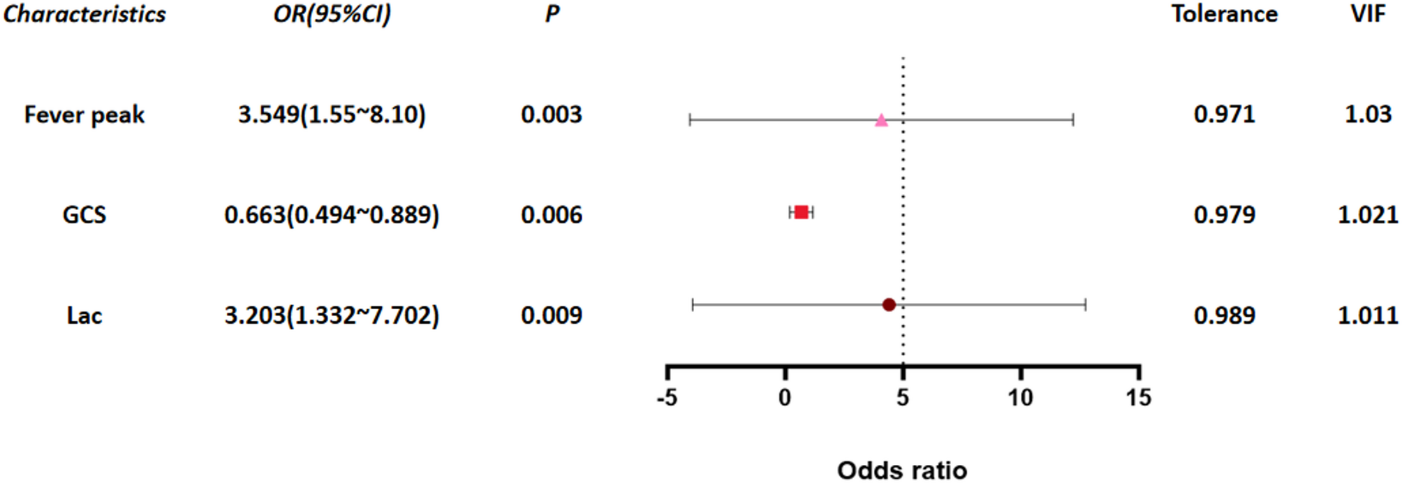
High fever, low GCS, and high lactate: independent risk factors for progression of influenza-associated encephalopathy to acute necrotizing encephalopathy in children | BMC Infectious Diseases
Research subjects
This study is a retrospective case-control study. Data of 6,647 pediatric influenza patients treated at Wuhan Children’s Hospital Affiliated to Tongji Medical College of Huazhong University of Science and Technology from…
Continue Reading
-

BrowserStack Launches Issue Detection AI Agent That Brings Human Intelligence to Accessibility Testing
DUBLIN, Oct. 28, 2025 /PRNewswire/ — BrowserStack, the world’s leading software testing platform, launched its Accessibility Issue Detection Agent, a breakthrough addition to…
Continue Reading
-
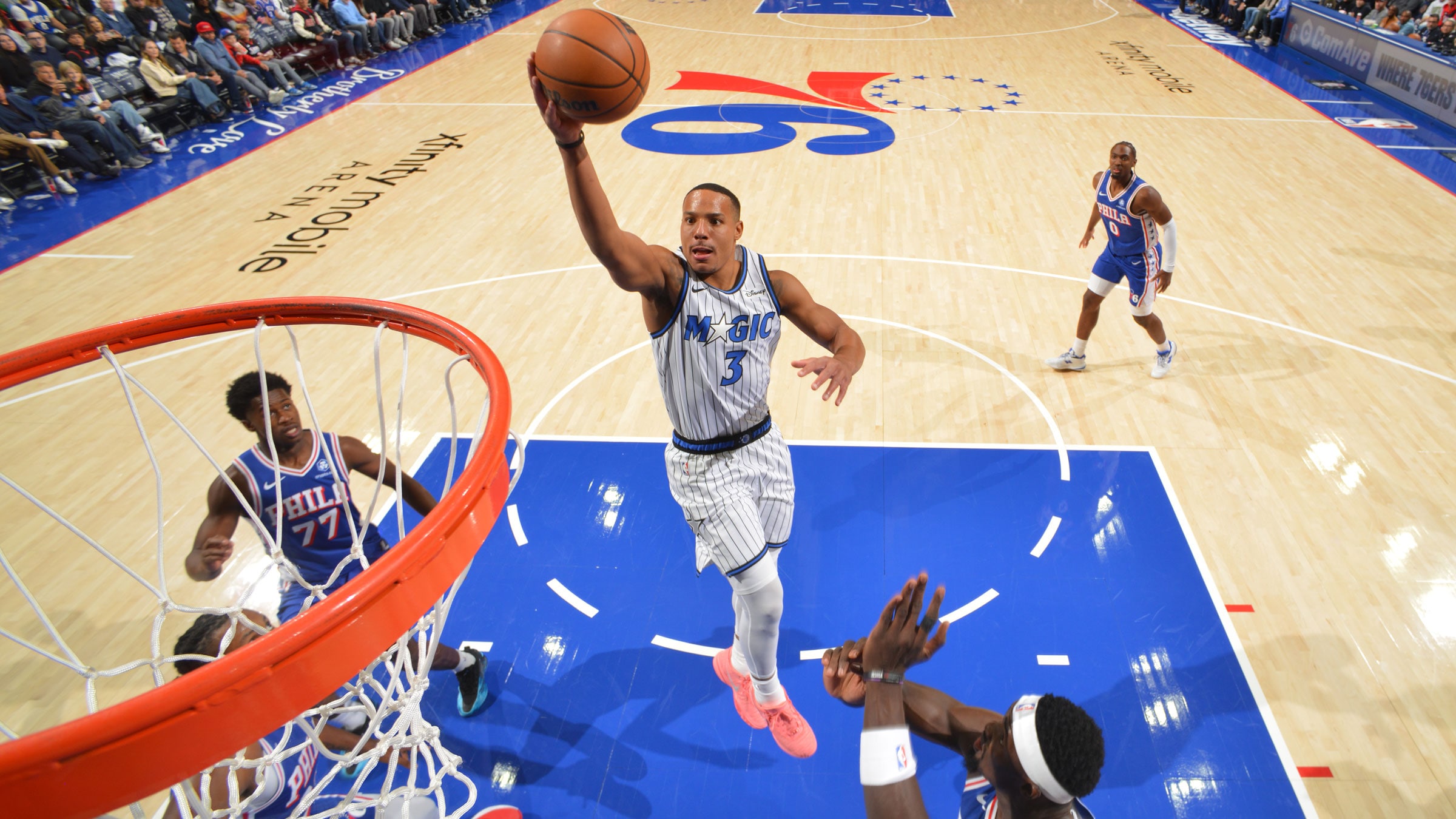
Quote & Analysis: Converting More in Crunch Time, Chemistry of Big Three, Free Throw Shooting & More – NBA
- Quote & Analysis: Converting More in Crunch Time, Chemistry of Big Three, Free Throw Shooting & More NBA
- Orlando Magic can’t allow surprisingly poor start to overshadow key improvement Orlando Magic Daily
- Orlando Magic’s struggles reflected in…
Continue Reading
-
Trump says seven ‘brand new, beautiful planes’ shot down during Pakistan-India war – Dawn
- Trump says seven ‘brand new, beautiful planes’ shot down during Pakistan-India war Dawn
- Diplomacy Over Dogfights: Trump’s Mediation And The Fragile Peace Between India And Pakistan – OpEd Eurasia Review
- Donald Trump says he spoke to PM…
Continue Reading
-
Estimating the contribution of musculoskeletal impairments to altered gait kinematics in children with cerebral palsy using predictive simulations | Journal of NeuroEngineering and Rehabilitation
Description of study participants
Data were collected for eight individuals with spastic CP planned for MLS at the time of their pre-operative clinical gait assessment (Table 1). Parents or caregivers signed an informed consent form, participants older than twelve signed an informed assent form. The study was approved by the Ethical Committee UZ/KU Leuven (S64909).
Table 1 Study participants Description of experimental data
All study participants had a clinical examination and 3D gait analysis followed by an MRI scan of the legs and pelvis.
Clinical examination
The clinical examination was performed by an experienced clinician. This examination was part of standard clinical care and was used to inform clinical decision making. It assessed muscle length, strength, bony alignment, and motor control. Muscle length was evaluated by passively moving the joints to the end of range of motion and measuring the final angle with a goniometer. Evaluated joint motions were hip flexion, hip extension, knee flexion, knee extension, ankle dorsiflexion, and ankle plantarflexion. Muscle strength was evaluated using modified Manual Muscle Testing (MMT). The strength of hip flexors, extensors, abductors and adductors, knee flexors and extensors, ankle plantar flexors and dorsiflexors, invertors and evertors was tested. When no muscle contraction could be palpated, the muscle group was scored 0, when the individual could move against gravity with maximal resistance the muscle group was scored 5 (Table S1 refers to supplement). A specific evaluation of abdominal and back muscles was also performed and scored between 0 and 5 (Table S2-S3). For alignment, femoral anteversion [21], bimalleolar angle and tibiofemoral angle [22] were evaluated. For motor control, both spasticity and selectivity were assessed. Spasticity was assessed using the modified Ashworth scale [23], Tardieu scale [24], and Duncan-Ely [22]. The Selective Motor Control Test [25] and Selective Control Assessment of the Lower Extremity [26] were used to evaluate selectivity.
3D gait analysis
The gait analysis was performed at a self-selected speed and marker trajectories were captured with a 12-camera Vicon system (Vicon, Oxford, UK; sampling frequency of 100 Hz). Markers were attached according to an extended lower limb plug-in gait model (Table S4). Ground reaction forces were collected at 1000 Hz with two embedded force plates (AMTI, Watertown MA, USA) in the raised 10-meter walkway. Muscle activity of eight muscles was measured bilaterally with a 16-channel telemetric surface electromyography system (Zerowire, Cometa, Italy) at 1000 Hz. The electrodes were placed according to the SENIAM guidelines [27]. In this study, we only evaluated and compared kinematics.
MRI
MRI of the lower limbs and pelvis were acquired similar to Bosmans et al. [28]. Depending on the individual’s size, three to five axial image series were acquired on a 3T Siemens MR scanner using a T1 weighted SE sequence with the participants lying supine with extended knees. For the image series containing the hip, knee, or ankle, inter-slice distance was 1 mm with a voxel size of 1.04 × 1.04 × 1 mm. For the other image series, the inter-slice distance was 2 mm with a voxel size of 1.04 × 1.04 × 2 mm. Glycerin markers were placed on the marker locations of the 3D gait analysis to ensure correct registration for inverse kinematics.
Predictive simulations
We performed predictive simulations of walking using PredSim [7, 29]. In short, we solved for the gait cycle duration, muscle controls, and the corresponding gait pattern by minimizing a cost function while imposing task constraints and musculoskeletal dynamics without relying on experimental gait data. The task constraints were an imposed average forward speed of the pelvis as well as periodicity. We prescribed the participants’ walking speed in the simulations. Since we did not explicitly model contact between limbs, we used distance constraints scaled based on body height to prevent segments penetrating each other. We used a previously determined cost function [7], i.e. the integral of the weighted sum of squared metabolic energy rate ((:dot{E})), muscle activations ((:a)), joint accelerations ((:{u}_{a}^{})), and passive joint torques ((:{T}_{p}^{})):
$$J=frac{1}{d}mathop smallint limits_{0}^{{{t_f}}} left( {{s_1}*{w_1}*{{dot {E}}^2}+{w_2}*{a^2}+{w_3}*u_{a}^{2}+~{s_4}*{w_4}*T_{p}^{2}} right)*dt$$
(1)
$${s_1}=~frac{1}{{left( {frac{{{M_{subject}}}}{{{M_{DHondt2024}}}}} right)*{{left( {frac{{{L_{subject}}}}{{{L_{DHondt2024}}}}} right)}^2}}}$$
(2)
$${s_4}={left( {frac{{{M_{DHondt2024}}*~{L_{DHondt2024}}}}{{{M_{subject}}~*~{L_{subject}}}}} right)^2}$$
(3)
where (:d) is the distance traveled, (:{t}_{f}) is gait cycle duration, (:t) is time, and (:{w}_{1}-:{w}_{4}) are weight factors, (:{M}_{subject}) is the mass of the subject, (:{L}_{subject}) is the height of the subject, and (:{M}_{DHondt{2024}_{}}) and (:{L}_{DHondt{2024}_{}}) are the mass and height of the generic model (described in detail below). Muscle metabolic energy was calculated using the model of Bhargava et al. [30], which was made continuously differentiable by approximating conditional statements with a hyperbolic tangent.
The resulting optimal control problems were solved using direct collocation (100 mesh intervals, 3 collocation points) and algorithmic differentiation. Problems were formulated and solved in MATLAB (R2021b, MathWorks Inc, Natick, Massachusetts, USA). Skeleton dynamics was formulated through OpenSimAD [31], CasADi [32] was used for problem formulation and algorithmic differentiation, and the resulting nonlinear programming problems were solved in IPOPT [33] (tolerance: 10−4). For each model, we used at least two initial guesses. The converged simulation with the lowest cost was chosen as final result.
Model personalization
We performed a series of simulations based on models with different levels of personalization to evaluate how musculoskeletal impairments affect the gait pattern. We divided the musculoskeletal impairments into muscle weakness, muscle contractures, and bony deformities. Muscle weakness and contractures were derived from the clinical examination. We derived bony deformities from the MR images using a previously developed approach to determine hip joint centers and knee axes as well as muscle-tendon paths of muscles spanning the hip and knee (but not the ankle) [13]. To investigate the contribution of these impairments as well as interaction effects, we created eight musculoskeletal models as described in Table 2.
Table 2 Model description Generic musculoskeletal model
All models were based on the model with a three-segment foot (talus, hindfoot-midfoot-forefoot, and toes) proposed by D’Hondt et al. [34]. The model has 31 degrees of freedom (DOFs) (pelvis-to-ground: 6 DOFs, hip: 3 DOFs, knee: 1 DOF, ankle: 1 DOF, subtalar: 1 DOF, metatarsophalangeal: 1 DOF, lumbar: 3 DOFs, shoulder: 3 DOFs, and elbow: 1 DOF). The lower limb and lumbar joints are actuated by 92 Hill-type muscle-tendon units [35, 36]. The MTP joint is actuated by a spring and damper. The shoulder and elbow joints are actuated by eight ideal torque actuators. Foot-ground contact is modeled by five Hunt-Crossley contact spheres per foot. Passive joint torques with exponential stiffness and damping [37] represent the effects of unmodeled passive structures in the lower limb and lumbar joints [7]. Muscle excitation-activation coupling was described by Raasch’s model [38, 39]. Skeletal motion was modeled with Newtonian rigid body dynamics [31, 40]. We removed quadratus femoris and gemellus because modeling bony deformities caused unrealistic operating ranges (>1.5 normalized fiber lengths) of these small muscles for some participants whereas removing both muscles from the generic model had little effect on the simulated gait pattern.
Reference model
The reference model (GEN) is the generic model described above scaled to the participant’s anthropometry using the OpenSim Scale Tool [9]. We additionally scaled maximal isometric force, which is not affected by scaling in OpenSim, based on subject mass [41]:
$$F_{{m,subject}}^{{max}}~=~F_{{m,DHondt2024}}^{{max}}*{left( {frac{{{M_{subject}}}}{{{M_{DHondt2024}}}}} right)^{left( {2/3} right)}}$$
(4)
with (:{F}_{}^{max}) the maximal isometric force and (:M) the mass of the respective models. Parameters of the foot-ground contact model, and stiffness and damping of the joints, were also scaled based on the subject’s anthropometry (equations S1–S4). This model does not include impairments, with exception of leg length differences and was used as the basis for further personalization.
Modeling muscle weakness
To model muscle weakness, active fiber force was scaled based on the MMT scores from the clinical examination:
$${F_m}=F_{m}^{{max}}*left( {sf*f_{m}^{{act}}left( {{{tilde {l}}_m}~,~{{tilde {v}}_m}~,a} right)+~f_{m}^{{pass}}left( {{{tilde {l}}_m}} right)} right)$$
(5)
where (:{F}_{m}) is muscle force, (:{F}_{m}^{max}) is the maximal isometric force, (:sf) is the weakness scale factor, (:{f}_{m}^{act}) is the active muscle force-length-velocity characteristic, (:{stackrel{sim}{l}}_{m}) is normalized fiber length, (:{stackrel{sim}{v}}_{m}) is normalized fiber velocity, (:a) is muscle activation, and (:{f}_{m}^{pass}) is the passive muscle force-length characteristic. The weakness scale factors were determined semi-arbitrarily. We performed preliminary simulations with different sets of scaling factors, which were chosen based on intuition about how MMT scores would translate to reductions in strength. For four out of the eight participants we performed simulations with two different scaling sets [1.0, 0.7, 0.5, 0.3, 0.2, 0.1] and [0.7, 0.5, 0.3, 0.2, 0.1, 0.05] for MMT scores of 5, 4, 3, 2, 1, 0 combined with either the same or larger reductions in strength for plantar flexors and selected the set for which weakness explained most of their gait deficits. This resulted in scale factors for active fiber force of 0.7, 0.5, 0.3, 0.2, 0.1, and 0.05 for MMT scores of 5, 4, 3, 2, 1, 0, respectively. For plantar flexors, we reduced the scaling factor by one step (e.g. a score of 3 corresponds to a scaling factor of 0.2 instead of 0.3). We then applied the same scaling set for all participants. We grouped muscles to link the MMT scores to individual muscles. Hip muscles were divided into abductors (gluteus minimus and medius, tensor fascia latea and piriformis), adductors (adductors and pectineus), flexors (iliacus and psoas) and extensors (gluteus maximus and biceps femoris long head). Knee muscles were divided into flexors (remaining knee flexors attaching on pelvis or femur) and extensors (quadriceps). Muscles spanning the ankle were divided into plantar flexors (gastrocnemius medialis, gastrocnemius lateralis, soleus), dorsiflexors (tibialis anterior and toe extensor muscles), evertors (peronei) and invertors (toe flexors and tibialis posterior).
Modeling muscle contractures
Muscle fiber lengths have been observed to be shorter in CP [42]. Therefore, we chose to model contractures in the Hill-type muscles by reducing optimal fiber length. When optimal fiber length is reduced, muscle fibers will be stretched more at the same muscle-tendon length resulting in higher passive forces.
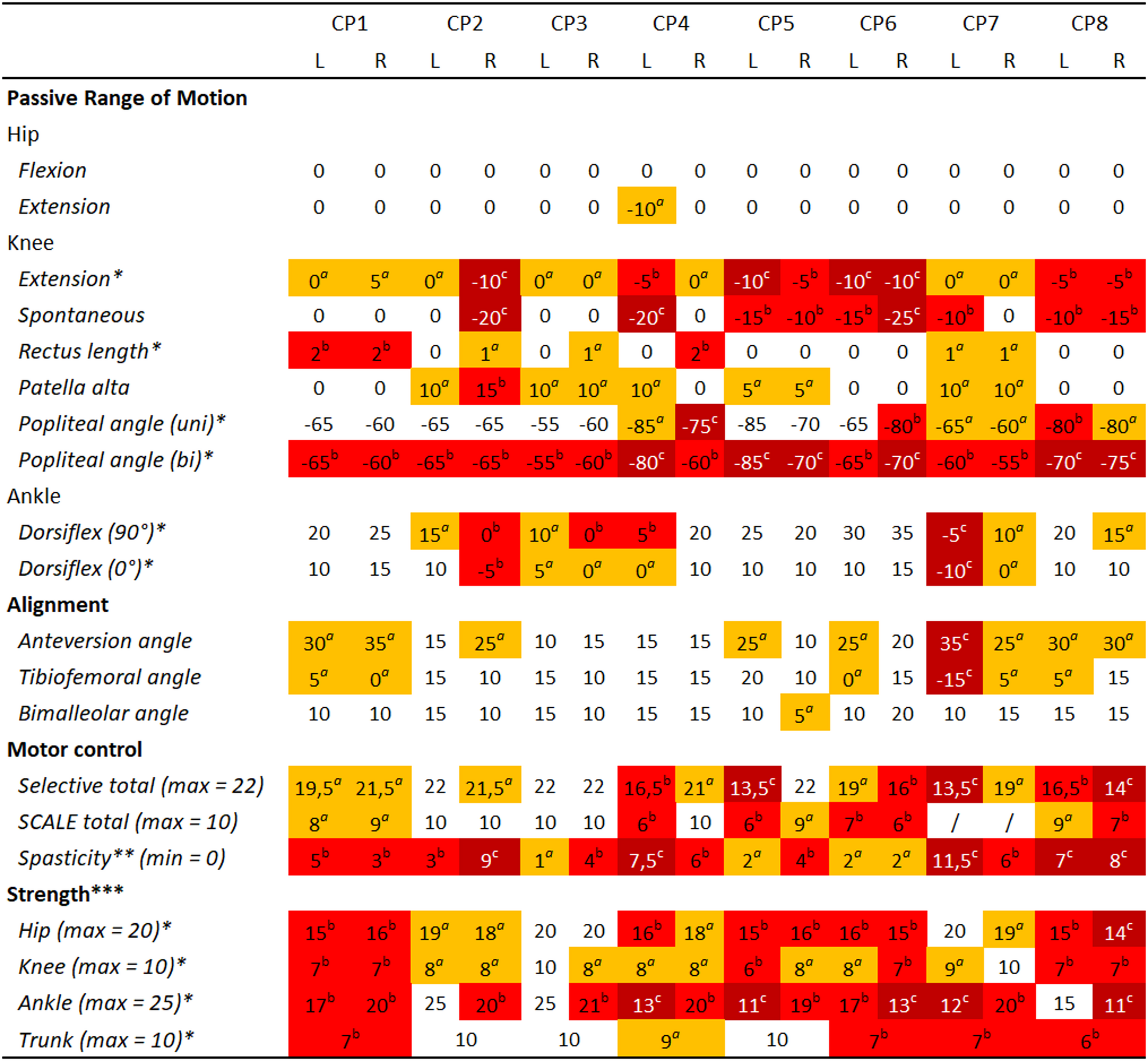
We only modeled contractures when there was a clinical indication (Fig. 1), i.e. clinical examination angles for passive range of motion were out of the typical range [43]. To determine the optimal fiber length for contracted muscles, we placed the musculoskeletal model in the same position as during the passive range of motion assessment and activated the muscle to 1%. We then determined the optimal fiber length such that the net modeled joint torque was 15 Nm at the end of range of motion.
Fig. 1 Clinical examination. Measured values were categorized with aslight impairment (orange), bconsiderable impairment (red) and csevere impairment (dark red) based on the data of the eight participants and the normative values [43] to aid with interpretation of the results. No categorization means the value is within normal range. Note that range of motion values indicate joint angles at end range of motion rather than deviations from values of typically developing individuals. * refers to values used for model personalization, ** refers to values from Modified Ashworth Scale, *** refers to the sum of different Muscle Testing Scores of muscles spanning the joint,/refers to no values recorded during the clinical examination. Tables with all individual values from the clinical exam can be found in the supplementary material (Table S5 for strength, Table S9 for motor control)
Soleus length was scaled based on maximal dorsiflexion angle with the knee flexed to 90°. The gastrocnemii length was scaled based on maximal dorsiflexion angle with the knees fully extended. Knee flexor length was scaled based on the bilateral popliteal angle. We used the same scaling factor for all knee flexors, i.e. biceps femoris long head, semimembranosus, semitendinosus, gracillis and sartorius. To obtain scaling factors for rectus femoris, we translated the score of the slow Duncan-Ely test to fixed scaling factors since one score allows for a wide range of knee flexion angles. For score 0 scaling was 1, for score 1 scaling was 0.9, and for score 2 scaling was 0.8 of nominal optimal fiber length.
We used a different approach to model iliopsoas contractures as their assessment is different. Iliopsoas contractures will lead to a different uni- ((:{theta:}_{uni})) and bilateral ((:{theta:}_{bi})) popliteal angle, that is the knee angle at maximal extension when the individual is supine with the thigh of the evaluated limb or both thighs vertical. When assessing the unilateral popliteal angle, the contralateral leg is laying down. Iliopsoas contractures will cause flexion of the contralateral hip and this will be compensated for by anterior pelvis tilt, which in turn will lead to increased hip flexion to position the thigh of the evaluated leg vertically. Increased hip flexion will in turn increase bi-articular hamstrings length and will thus lead to a larger knee extension deficit. The increase in hip flexion angle was determined based on the difference in popliteal angles and the ratio of the average moment arms of all bi-articular hamstrings with respect to the knee and hip:
$$Delta {theta _{hip}}=left( {{theta _{bi}} – ~{theta _{uni}}} right)*frac{{mathop sum nolimits_{{i~=~1}}^{n} ~frac{{m{a_{knee,i}}}}{{m{a_{hip,~i}}}}}}{n}$$
(6)
with n the number of bi-articular hamstrings, and (:{ma}_{knee,i}) and (:{ma}_{hip,i}) the moment arm of muscle i around knee and hip when in the position of the bilateral popliteal angle. We then determined the contracture of the contralateral iliopsoas by solving for the scaling factor that led to passive torque when the contralateral hip was extended beyond (:varDelta:{theta:}_{hip}).
Observed knee extension and plantar flexion deficits were modeled by shifting the coordinate limit torques that model the stiffness of the non-muscle soft tissues around the joint. For the knee, we shifted the limits such that torque started to develop at the observed angle for knee extension minus two degrees to obtain around 15 Nm torque at end range of motion. We modeled plantar flexion deficits based on the reported range of motion for the ankle towards plantar flexion. The onset of the coordinate limit torques was changed to 25° plantar flexion or 0° when the score was respectively ‘discrete’ or ‘severe’.
Modeling bony deformities
Bony deformities were modeled based on the MR images. First, bones were segmented with Materialise Mimics (Materialise, Leuven, BE). Further processing was performed in MuscleSegmenter [13]. We determined the pelvic frame based on anatomical landmarks of the pelvis and located the glycerin markers. Next, the hip joint center was estimated by fitting a sphere to the femoral head. Then, reference frames of the femur, patella and tibia were determined based on anatomical landmarks. Next, the knee joint axis was determined based on fitting two ellipsoids to the condyles and visual inspection (congruence of joint contact surfaces) of the knee motion. Next, the paths of muscles spanning the hip and knee as well as the attachment points of the gastrocnemii on the femur were segmented. Muscle paths were chosen such that they approximated the centroid of the muscle belly. Next, the scaled generic model was updated by replacing the original joint centers, marker locations, and muscle paths by the values obtained from the MR images followed by linear scaling of optimal fiber lengths and tendon slack lengths (similar to the OpenSim Scale Tool) through a custom-made MATLAB (R2021b, MathWorks Inc, Natick, Massachusetts, USA) script.
Strength deficits observed during MMT can be due to both moment arm deficits or reduced muscle force generating capacity. The MRI-informed models already capture weakness due to moment arm deficits. Therefore, we modified the weakness scale factor derived from MMT to correct for weakness due to moment arm deficits:
$$s{f_{geo}}=sf*~{left( {frac{{T_{{max}}^{{GEO}}}}{{T_{{max}}^{{GEN}}}}} right)^{ – 1}}$$
(7)
with (:{sf}_{geo}) the corrected weakness scale factor to be used in the model with bony deformities, (:sf) the weakness scale factor derived from MMT, (:{T}_{max}^{GEN}) the maximal torque the muscle group could generate in the GEN model, and (:{T}_{max}^{GEO}) the maximal torque the muscle group could generate in the GEO model. The ratio between(::{T}_{max}^{GEO}) and (:{T}_{max}^{GEN}) thus reflects the moment arm deficit (Table S8). (:{T}_{max}^{}) was evaluated with the model in the same position as during MMT and agonist muscles activated to 100%.
Since muscle-tendon paths differ in the GEO model compared to GEN, we estimated contractures in both models separately.
Outcome measures and statistical analysis
Experimental kinematics were calculated from marker trajectories collected during walking at self-selected speed based on the GEO model with OpenSim’s Inverse Kinematics Tool. Means and standard deviations of the experimental gait were calculated based on five to ten strides per side. Walking speed was determined based on the average forward speed of the posterior pelvis marker over at least four strides.
Root Mean Square Differences (RMSD) and Pearson correlations (r) were calculated between simulated and mean experimental kinematics for hip flexion, hip adduction, hip rotation, knee flexion and ankle dorsiflexion. We calculated the mean RMSD and correlation over all sagittal and non-sagittal plane degrees of freedom for each subject-model pair. Differences in median and interquartile range (IQR) between GEN and the other models were used to interpret the contribution of the modeled impairments to the altered gait. The minimal important difference for RMSD was defined to be 1.6° [44]. We deemed differences in correlation of 0.05 practically relevant for this study.
We tested whether personalized models better captured the experimental data than the generic model (GEN) using SPM1D [45] to analyze differences in the deviation of simulated from experimental kinematics between GEN and each of the personalized models. We used the paired t-test from the SPM1D Matlab package with two-tailed inference at alpha 0.05 [46]. We performed the analysis for each degree of freedom separately, but we combined trajectories from left and right legs. As our study design resulted in many different models to assess contributions of different impairments, the statistical analysis should be considered exploratory, i.e. we did not correct for multiple comparisons. We reported the statistical parametric map of t-values (SPM{t}) as well as p-values over intervals where the agreement between modeled and simulated kinematics differed between models (Figs. S4, S5) .
We determined the contribution of impairments to RMSD and correlations between simulated and experimental gait kinematics using Shapley values [47]. We computed Shapley values to quantify the contribution of weakness, contractures, bony deformities and any combination of two of these impairments. Shapley values are a weighted average of the marginal contribution of an impairment or set of impairments across all model combinations that differ in the impairments under investigation. Marginal contributions with respect to the generic model and fully personalized model are weighed more heavily (see supplement Sect. 9 for additional information).
Continue Reading
-

Govee’s new outlet expander gives you voice control and a night light
Did you know you should be replacing your surge protectors every three to five years to avoid them becoming a potential fire risk? If you’re now on the hunt for replacements, Govee’s new Smart Plug Outlet Extender packs a decent amount of…
Continue Reading
-

COVID-19 pandemic linked to diminishing public trust in childhood vaccines
An international study led by the Azrieli Faculty of Medicine in the Galilee at Bar-Ilan University reveals that the COVID-19 pandemic has contributed to a diminishing public trust in childhood vaccines, resulting in declining…
Continue Reading