Blog

Llama immunization and nanobody library construction

For nanobody generation, a recombinant murine LYVE1 protein, consisting of 288 amino acids, fused to a His10 tag, was expressed in human embryonic kidney 293 cells. The recombinant protein was injected alongside Adjuvant P (3111, GERBU Biotechnik GmbH, Heidelberg, Germany) weekly on six consecutive occasions into a Ilama (Lama glama). Forty days after the initial immunization, 100 mL of anticoagulated blood were collected from the Ilama, 5 days after the final antigen injection. Peripheral blood lymphocytes were isolated and total RNA extracted for cDNA first-strand synthesis using oligo(dT) primers. Sequences encoding variable nanobodies were subsequently amplified by PCR, digested with the restriction enzyme SapI, and cloned into the SapI site of the phagemid vector pMECS. Electrocompetent E. coli TG1 cells (60502, Lucigen, Middleton, WI, USA) were then transformed with the variable domain of heavy-chain-only antibody (VHH) sequence harbouring pMECS vectors, resulting in a nanobody library comprising 10⁹ independent transformants. This process has previously been described in detail [34].

Biopanning and identification of anti-mouse nanobodies specific to LYVE1

Phage enrichment and biopanning were carried out as described [34]. Briefly, the previously constructed nanobody library was panned for 3 rounds on solid phase coated with mouse LYVE1 (100 µg/mL in 100 mM NaHCO₃, pH 8.2) yielding a 400-fold enrichment of antigen-specific phages after the 3rd round of panning. A total of 380 colonies were randomly selected and assayed for mouse LYVE1-specific antigens by ELISA, again using mouse LYVE1 and additionally mouse LYVE1 fused to human IgG1 Fc at the C-terminus (50065-M02H, Sino Biological, Beijing, China). To exclude potential nanobody clones binding to human IgG1 Fc, human IgG1 Fc (10702-HNAH, Sino Biological) was utilized as a control, as well as blocking buffer only (100 mM NaHCO₃, pH 8.2). After comparing binding specificity of different clones with the control values, 278 colonies were identified as positive for mouse LYVE1 binding. Using the sequence data, the number of possible nanobody candidates was further narrowed down to 98, of which 96 were able to specifically bind both mouse LYVE1-His10 and mouse LYVE1 fused to human IgG1 Fc. The remaining unique clones derived from 21 different B cell lineages according to their complementary determining region (CDR) 3 groups. Considering the different B cell linages and robustness of ELISA screening data, 6 clones were selected for further experiments.

Cloning of nanobody sequences in expression vector

To generate 6xHis-tagged nanobodies, nanobody sequences were cloned from the pMECS phagemid vector into the pHEN6c expression vector. Initially, nanobody sequences were amplified by PCR using the following primers:

(1) 5’ GAT GTG CAG CTG CAG GAG TCT GGR GGA GG 3’.

(2) 5’ CTA GTG CGG CCG CTG AGG AGA CGG TGA CCT GGG T 3’.

PCR products were purified (28104, QIAquick PCR Purification Kit,, Qiagen, Hilden, Germany) and digested for 20 min at 37 °C with PstI-HF (R3140, New England Biolabs, Ipswich, MA, USA) and BstEII-HF (R3162, New England Biolabs) restriction enzymes, while empty pHEN6c plasmids were concurrently digested with the same restriction enzymes. The empty pHEN6c plasmids, however, were supplemented by 5 units of heat-inactivated (5 min at 80 °C) FastAP™ alkaline phosphatase (EF0651, Thermo Fisher Scientific, Waltham, MA, USA). Digestion products were purified (28104, QIAquick PCR Purification Kit, Qiagen) and subjected to T4 DNA ligase-mediated ligation reactions. The ligation reaction was performed at 16 °C for 16 h using 2.5 units of T4 DNA ligase (M0202, New England Biolabs). Subsequently, newly generated nanobody sequence harbouring pHEN6c plasmids were transformed into WK6 E. coli cells (C303006, Thermo Fisher Scientific) and analysed to determine correct nanobody sequence integration by Sanger DNA sequencing using the following primers:

(1) 5’ TCA CAC AGG AAA CAG CTA TGA C 3’.

(2) 5’ CGC CAG GGT TTT CCC AGT CAC GAC 3’.

Production and purification of anti-LYVE1 nanobodies

WK6 E. coli carrying pHEN6c-Nanobody plasmid were cultivated at 37 °C, shaking in 1 L `Terrific Broth` medium (2.3 g/L KH₂PO₄, 16.4 g/L K₂HPO₄-3H₂O, 12 g/L tryptone, 24 g/L yeast extract, 0.4% (v/v) glycerol) complemented with 100 µg/mL ampicillin, 2 mM MgCl₂, and 0.1% (w/v) glucose. Nanobody expression was induced at an OD600 of 0.6–0.9 by adding 1 nM isopropyl ß-D-1-thiogalactopyranoside (IPTG). After an incubation period of 16 h, the nanobodies were extracted by centrifugation (8000× g, 8 min, RT). 18 mL of TES/4 buffer (0.05 M Tris [pH 8.0], 0.125 mM EDTA, 0.125 M sucrose) were added for 1 h of shaking on ice. The cell suspension was then centrifuged (8000× g, 30 min, 4 °C), and periplasmic protein-containing supernatant collected. For 6xHis-tagged nanobody extraction, HIS-Select^® nickel affinity gel (P6611, Sigma-Aldrich, Darmstadt, Germany) was applied according to the manufacturer’s instructions. The solution was loaded on a PD-10 column (17-0435-01, GE healthcare, Chicago, IL, USA) and nanobodies eluted via 3 × 1 mL 0.5 M imidazole in phosphate-buffered saline (PBS) (I2399, Sigma-Aldrich). An overnight dialysis (3 kDa MWCO, 66382, Thermo Fisher Scientific) against PBS was carried out to remove undesirable imidazole from the nanobody solution.

Coomassie-blue stained SDS PAGE and Western blotting

To verify nanobody production and pureness, sample protein was separated by molecular weight using established sodium dodecyl sulphate-polyacrylamide gel electrophoresis (SDS-PAGE). For each clone, 5 µg of denatured protein with 0.04% (w/v) OrangeG in ddH₂O) were loaded onto the gel alongside a pre-stained protein ladder (ab116029, Abcam, Cambridge, UK). For protein visualisation, gels were treated with Coomassie staining solution (0.1% (w/v), Coomassie Brilliant Blue R-250 (1610400, Bio-Rad Laboratories Inc., Hercules, CA, USA), 50% (v/v) methanol, and 10% (v/v) glacial acetic acid in ddH₂O for 1 h, followed by incubation with Coomassie destaining solution (50% ddH₂O, 40% methanol, 10% acetic acid (v/v/v)). Alternatively, gels were blotted onto a nitrocellulose membrane (1620112, Bio-Rad Laboratories Inc.) and nanobodies identified using a primary anti-His antibody (12698, Cell Signaling Technology, Danvers, MA, USA) and a secondary anti-rabbit antibody (926-32211, LI-COR Biosciences, Lincoln, NE, USA). Subsequently, blots were analysed by an Odyssey^® Fc Imaging System (LI-COR Biosciences).

Mouse husbandry and acquisition of mouse tissues

C57BL/6 wildtype mice, or Lyve1^{Cre − eGFP} mice [35] on the C57BL/6 background were utilised in this study. All animal experiments were carried out under a UK Home Office project license (PPL: PP1776587) in compliance with the UK Animals (Scientific Procedures) Act 1986 or approved by German federal authorities (LaGeSo Berlin) under the licence number ZH120. Nutrition and water were available to animals ad libitum. Mouse embryos were staged by time-matings, considering embryonic day (E) 0.5 to be the morning a copulation plug was detected. Adult mice or pregnant mice were sacrificed using CO₂ inhalation and cervical translocation as a Schedule 1 procedure. The desired organs were obtained from embryonic, juvenile, or adult mice, washed in PBS, and subsequently fixed in 4% (w/v) paraformaldehyde (PFA) in PBS for 4 h at 4 °C to preserve tissue integrity. After fixation, samples were thoroughly washed in three changes of PBS and stored at 4 °C in PBS containing 0.03% (w/v) sodium azide until further processing.

Antibodies for Immunofluorescence

The following commercially available antibodies were used: rabbit monoclonal anti-His antibody (12698, Cell Signaling Technologies) [1:200], donkey polyclonal anti-rabbit IgG Alexa Fluor™ 647 antibody (A31573, Invitrogen, Waltham, MA, USA) [1:1000], donkey polyclonal anti-rabbit IgG Highly-Cross-Absorbed Alexa Fluor™ 647 antibody (A32795, Invitrogen) [1:1000], goat polyclonal anti-mLYVE1 (AF2125, R&D Systems, Minneapolis, MN, USA) [1:100], donkey polyclonal anti-goat IgG Alexa Fluor™ 568 antibody (A11057, Invitrogen) [1:1000], donkey polyclonal anti-goat IgG Highly cross-absorbed Alexa Fluor™ 488 + antibody (A32814, Invitrogen) [1:1000], hamster monoclonal anti-Podoplanin (14-5381-82, Invitrogen) [1:200], goat polyclonal anti-Syrian hamster IgG Cross-Absorbed Alexa Fluor™ 546 antibody (A-21111, Invitrogen) [1:1000], chicken polyclonal anti-GFP (ab13970, Abcam) [1:200], donkey anti-chicken Highly cross-absorbed Alexa Fluor™ 488 + antibody (A32931TR, Invitrogen) [1:1000], rat monoclonal anti-mF4/80 antibody (MCA497G, BioRad) [1:50], donkey anti-rat Highly cross-absorbed Alexa Fluor™ 488 + antibody (A48269, Invitrogen) [1:1000]. Nanobodies were detected by anti-His staining in combination with an Alexa Fluor™ dye-conjugated secondary antibody. An overview of antibody combinations used for each experiment including concentration and incubation time can be found in Table S1.

Zenon labelling of IgG antibodies

Anti-His antibodies were labelled using the Zenon™ Rabbit IgG Labeling Kit (Z25306, Thermo Fisher Scientific) by incubating the antibody with Component A for 5 min, followed by blocking with Component B for another 5 min. The labelled antibody was used within 30 min.

Direct labelling of nanobodies

Anti-mouse LYVE1 nanobodies were directly labelled with Alexa Fluor™ 647 NHS-Ester (A20006, Invitrogen) by reacting 1 mg of nanobody with 1 mg of dye in NaHCO₃ buffer (pH 8.0) for 1 h at room temperature. Labelled nanobodies were purified using a NAP™-10 column (Sephadex™ G-25, Thermo Fisher) and stored in PBS with 0.03% (w/v) sodium azide.

Immunofluorescence staining of cryosections

Snap-frozen 5 μm sections of E14.5 wildtype mice were stained with nanobodies (0.1 µg/mL) and appropriate control antibodies as previously described [36]. Visualisation of representative regions was accomplished using an Axioscope5 fluorescence microscope (Zeiss, Oberkochen, Germany) equipped with a Plan-NEOFLUAR 40x/0.75 objective (Zeiss).

Wholemount Immunofluorescence staining and optical clearing

Mouse organs were either cut into smaller sections measuring 0.5–2 mm thickness (for studies in Figs. 2A, 3 and 4, Fig. S3B) using a scalpel at room temperature or processed as whole specimens (for studies in Figs. 2B and 4A (E18.5-P5), Fig. S3A, Fig. S4). Tissues were dehydrated using an ascending methanol series and bleached overnight at 4 °C in a solution containing 5% H₂O₂ (VWR Chemicals, Radnor, PE, USA) in methanol. Wholemount staining was performed as previously described [22]. For optical clearing, samples were treated with methanol for dehydration followed by BABB (1:2 benzyl alcohol and benzyl benzoate) immersion, as described in [22]. Intestine samples were not optically-cleared, but mounted in fluorescent medium (S3023, Agilent Technologies, Santa Clara, CA, USA). Details on antibodies used, incubation periods and concentrations are outlined in Table S1.

Wholemount Immunofluorescence staining and optical clearing of embryonic and postnatal day one specimens

Embryonic and early postnatal (P) kidneys were initially dehydrated and bleached as described above. Following rehydration, samples were permeabilized overnight in a 5% solution of 3-((3-cholamidopropyl) dimethylammonio)-1-propanesulfonate in ddH₂O and blocked in PBS supplemented with 0.2% (v/v) Triton X100, 10% (v/v) DMSO, and 6% (v/v) goat serum. Nanobodies (10 µg/mL) and antibodies were diluted in antibody solution (PBS + 0.2% v/v Tween20 + 0.1% v/v heparin solution + 5% v/v DMSO + 3% v/v goat serum + 0.1% w/v saponin) and incubated for a duration between 4 (nanobodies) and 24 h (IgG antibodies) at 4 °C. Between staining steps, samples were washed in PBS-Tween20. Clearing was performed with BABB as previously described for embryonic kidneys [37].

Confocal and light sheet imaging

Specimens were imaged using two different microscopy systems. For confocal imaging, an LSM 880 Upright Confocal Multiphoton microscope (Zeiss) equipped with a 20x/NA 1.0 W-plan Apochromat water immersion objective was utilized. A comprehensive description of the setup specific to BABB-cleared specimens for this microscope can be found in previously published work [37]. Intact mouse organs were imaged by LaVision Ultramicroscope II with a LaVison BioTec MVPLAPO 2x OC OBE objective. Various magnifications were employed, and image acquisition utilized a step size of 2 μm. Imaging thresholds were set individually for each channel during image acquisition and post-processing. This approach was chosen to accommodate the variability in autofluorescence and other factors, and to ensure optimal signal detection for each channel.

Image processing and 3D rendering

2D immunofluorescence images were subjected to post-processing using ZEN 3.4 (blue edition) software from Zeiss. Single channels were extracted and saved in TIFF format. Z-stack datasets were processed and 3D-rendered using Imaris (version 9.8, Oxford Instruments Abingdon, UK). To reduce non-specific background signal, single channels were subjected to the Isosurface Render function. Images of the 3D-rendered data were captured using the Snapshot function and saved in TIFF format. Videos were captured using the Animation function.

Quantification of signal-to-background ratio

Signal-to-background ratio was quantified using ImageJ 2.24/1.54f (https://github.com/imagej/ImageJ [38]), . Ten intensity values were randomly selected in vessel areas and areas that showed no specific staining. The mean values for signal and background areas were calculated and the signal-to-background ratio was determined using the formula: Signal-to-background ratio = mean signal/mean background.

Calculation of correlation coefficients

Pearson’s correlation coefficients r were calculated using the Imaris Coloc function. For very large microscopy files, colocalization analysis was performed on representative regions of interest, as full-volume analysis was not computationally feasible on the available hardware. For colocalization of nuclear GFP staining and endothelial nanobody staining, an object-based approach was applied. Spots were segmented independently for GFP and LYVE1 signals using the Imaris Spots function. For each LYVE1 spot, the shortest distance to the nearest GFP spot was determined. LYVE1 spots within 25 μm of a GFP spot were classified as colocalized, and the coefficient was calculated as the proportion of colocalized LYVE1 spots relative to the total number of LYVE1 spots.

Quantitative analysis of 3D imaging volumes

The quantitative analysis of three-dimensional volumes commenced with the binarization of single channels using Imaris. The binarization process was conducted using the Isosurface Render function, and for E18.5 and P1 samples, 3D cropping was applied to exclude regions with high podoplanin (PDPN) intensity at the kidney surface, thus enhancing binarization accuracy. During surface rendering, the threshold was set to absolute intensity, with manual adjustments to ensure the inclusion of all relevant structures. To eliminate smaller non-specific signals, structures were filtered based on the number of voxels. Following surface generation, PDPN channel-derived non-lymphatic structures, such as glomeruli, were manually removed using the selection function. Subsequently, the channel of interest was masked using specific settings: constant inside/outside, setting voxels outside the surface to 0.00, and inside the surface to the maximum intensity of the prepared channel. All channels except the newly created masked channel were then deleted, and the single channel was saved in TIFF format. With the binarized files prepared, TIFF files were imported into the VesselVio application [39]. The analysis settings were configured as follows: unit µm, resolution type anisotropic with individual sizes of samples, analysis dimensions 3D, image resolution 1.0 µm³, and filters applied to isolate segments shorter than 10.0 µm and purge end-point segments shorter than 10.0 µm. Analysis results were automatically saved in Microsoft Excel files by VesselVio. Among the parameters offered by VesselVio, vessel volume was selected as the parameter for further analysis, as it considers both vessel length and width. To account for variability in sample size and volume, vessel volumes (LYVE1 and PDPN) were normalized by dividing the measured vessel volume by the total sample volume, calculated based on the Imaris output for the x, y, and z dimensions. This normalized value was referred to as ‘relative volume’ [40].

Single-cell RNA sequencing analysis

The generation of the mouse kidney scRNA-seq data used in this study has been described [41]. In brief, a regional enrichment strategy was used to isolate hilum, cortex and medulla separately from 12-week-old C57Bl/6 mouse kidneys (n = 14), before single-cell droplet capture using the 10X Genomics platform (10x Genomics, Pleasanton, USA) and sequencing using an Illumina HiSeq X system (San Diego, USA). The count matrix corresponding to the lymphatic cluster was isolated and re-processed, applying a standard workflow using Seurat (v5) in R [42]. The Harmony package [43] was used for integration, using the mouse identifier as a batch variable. Differential expression analysis was performed using the FindAllMarkers function, utilising Wilcoxon rank sum tests. Marker genes are presented with average log-fold change (log2FC) values and an adjusted p value of < 0.05 was considered as statistically significant. Gene ontology (GO) analysis was applied using the Panther database [44], using statistical overrepresentation tests and calculating the false discovery rate (FDR) for each GO term.

Sample size Estimation and statistical analysis

Sample size was estimated based on prior publications of developmental studies of kidney lymphatic vessels [40] and studies investigating lymphatics in adult mice organs [9, 16]. These indicated that 6–8 animals per experiment would be sufficient to power statistical analyses. Statistical analysis was conducted using Prism (v8, GraphPad by Dotmatics, Boston, MA, USA) and RStudio version 12.0 (Posit, Boston, MA, USA). To determine the significance of differences in volume between LYVE1 and PDPN at individual time points and individual organs, a paired student’s t-test was carried out. For comparisons of Pearson correlation coefficients r, one-way ANOVA followed by Tukey’s post hoc test was applied. To assess statistical significance across different time points a rank-based approach using the R package nparcomp [45] with the function mctp1 (multiple comparisons for relative contrast effect testing) was chosen. This approach allows for nonparametric multiple comparisons to evaluate relative contrast effects. A p value of less than 0.05 was considered statistically significant for all tests. Quantitative data was visualised using Prism. All graphical representations present individual data points either by region of interest or by animal, along with the mean and standard error of the mean.

Preparation of figures and videos

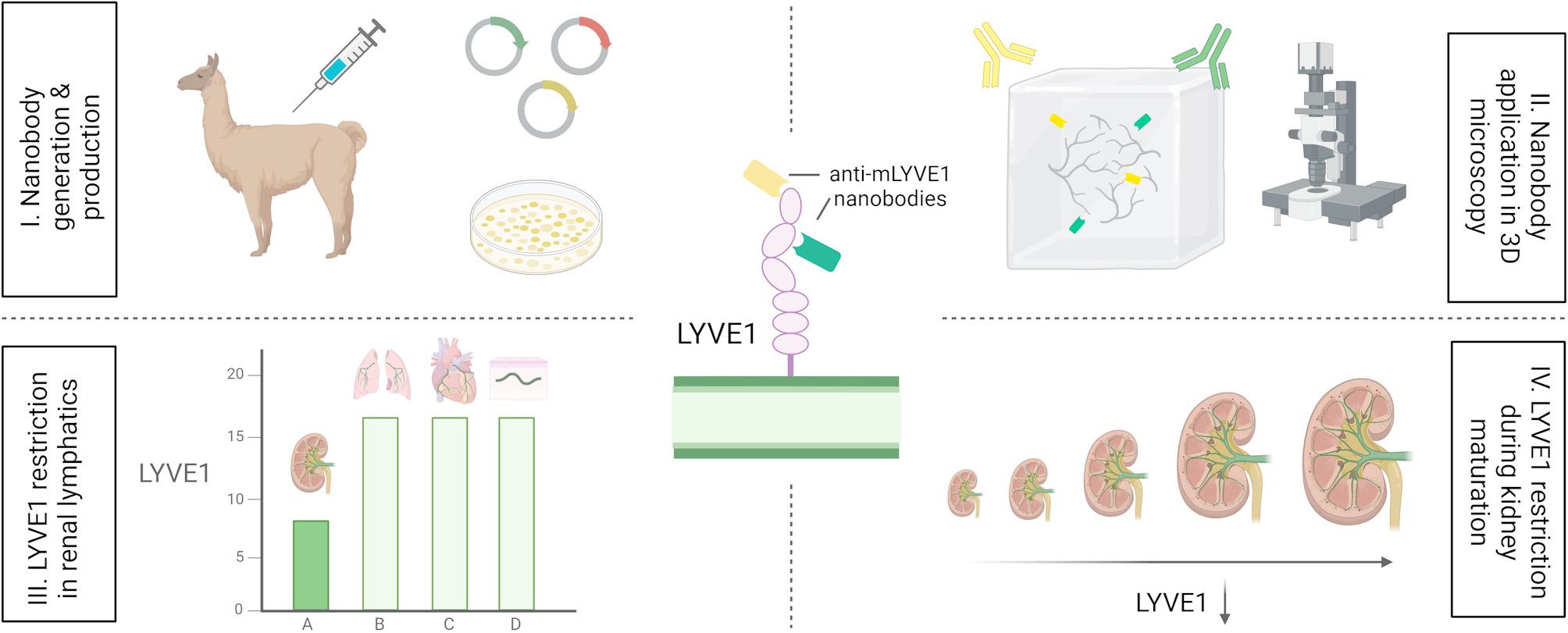
The graphical abstract was created in BioRender.com. The figures presented in this paper were prepared using the free software tool Inkscape 1.1.0 (Inkscape Project, 2020) for graphic design and layout. Any modifications made to the images, such as adjustment of brightness and contrast, were applied consistently throughout one panel to maintain uniformity across all coherent single and merged channel images. Videos were edited in Clipchamp (Microsoft, Redmond, WA, USA).

The Chinese online marketplace Temu’s EU operations more than doubled pre-tax profits last year to just below $120m (£90m) despite employing just eight people, accounts show.

They rose 171% in the 12 months to December 2024 compared with the $44.1m the year before, as shoppers snapped up its low-cost goods, which are widely promoted on social media.

However, the company paid just $18m in corporation tax, almost $3m of which was a mandatory top-up tax brought in at the end of 2023 after the EU signed up to a global minimum tax rate for large companies.

The accounts filed for the group’s Ireland-based EU parent group, Whaleco Technology, also show revenues rose to $1.7bn, compared with $758m the previous year, before new controls on the super-budget retailer.

Separate documents show Temu now has more than 115 million customers across the EU – equivalent to more than a quarter of the population.

The figures emerged after separate accounts showed almost doubling profits and revenues at the online marketplace’s UK operations.

The rise in sales comes before moves by the EU to close a loophole that allows packages worth less than €150 (£130) to avoid customs duty and some border checks.

Last year, 4.6bn low-value parcels entered the EU, equivalent to 12m a day, three times more than in 2022. More than 91% of parcels valued at less than €150 came from China, where Temu and its fellow low-cost seller Shein make and dispatch most of their goods.

However, controls began to be tightened in July this year, and customs duty is expected to be applied from 2028.

The US this summer abolished its “de minimis” exemption, which allowed goods worth less than $800 to skip import duty, to limit the rise of Temu and Shein, while the UK chancellor has said she is reviewing a similar loophole.

Paul Monaghan, the chief executive of the Fair Tax Foundation, estimates that Temu’s Irish entity facilitated consumer sales of $10bn in the EU – as its revenue figure only accounts for the company’s commission and fees from independent sellers on its marketplace.

If Temu’s estimated $2bn in sales via its sellers are included in the UK, that would make the marketplace bigger than the UK retailer Next and about the same size as Primark.

“Serious questions need to be asked as to why Temu has such a negligible economic and tax footprint in the UK and across Europe despite its enormous sales,” Monaghan said.

“What we have here is a chain of companies in a series of tax havens, that have been structured so as to leave little or no tax benefit in Europe.

skip past newsletter promotion

after newsletter promotion

“The UK and other European governments need to move much more quickly to not only protect their tax base, but allow existing retailers to compete on a level playing field with these Chinese e-commerce giants that have overseas tax avoidance hard-wired into their structures.

“Standing strong on the global minimum tax and digital services tax, reviewing customs duty exemptions and bolstering requirements for multinationals to publish a country-by-country breakdown of the taxes they pay would be a great place for politicians to start.”

A spokesperson for Temu said its operations in Ireland were “real operating companies employing real people” and the employee numbers did not reflect the full scale of its operation presence.

“Temu categorically rejects any suggestion that our structure or operations are designed to avoid taxes or minimise our economic footprint in Europe. Despite being a young and fast-growing company still in the investment phase, we have already paid billions of euros in taxes across European jurisdictions, and that figure will continue to rise as our operations mature.

“The tax figure cited refers only to the tax paid by a single legal entity and does not include customs duties, VAT, and other taxes.

“Temu entered the European market just two years ago and has invested heavily in building its platform to connect sellers and consumers more efficiently, passing those efficiencies back to consumers in the form of lower prices on quality goods. At the same time, we have been creating new growth opportunities for local sellers across Europe.

“Our focus is on the long term: building a sustainable, compliant, and trusted platform that helps consumers access quality products at affordable prices while enabling local sellers across Europe to grow their businesses and reach new markets.”

Efforts to leverage the immunomodulatory effects and synergistic combinability of CELMoDs like iberdomide (CC-220) and mezigdomide (CC-92480) to augment standard T-cell redirection therapies could lead to more durable remissions or even cures for patients with relapsed/refractory multiple myeloma, according to Joshua Richter, MD.¹

Preclinical data suggest that these CELMoDs, which operate through targeted degradation of the cereblon protein, could provide benefit to patients who are resistant to older drugs like lenalidomide (Revlimid) and pomalidomide (Pomalyst), providing a well-tolerated treatment that could be administered for longer durations and in combination with immune therapies or proteasome inhibitors.

“We are using these drugs to prime the collection [of T cells], and that may lead to higher curability using the CAR T-cell modality,” Richer shared in an interview with OncLive^® at the 22nd Annual International Myeloma Society Meeting and Exposition.

In the interview, Richter discussed how next-generation immunomodulatory drugs could enhance current T-cell therapies in myeloma, current avenues of investigation for CELMoDs in multiple myeloma, and the desired balance between outcomes and toxicity for future immune-based treatments in myeloma.

Richter is an associate professor of medicine in the Division of Hematology and Medical Oncology at The Tisch Cancer Institute, and director of Multiple Myeloma at Blavatnik Family Chelsea Medical Center, Mount Sinai, in New York.

OncLive: How might next-generation immunomodulatory drugs enhance current T-cell therapies in myeloma, and what is the ultimate goal of these combinations?

Richter: [There have been] 3 great epochs of treatment in myeloma. In the old days, we started with classical chemotherapy. Then we moved on to the second generation [of treatment], with novel agents like immunomodulatory drugs, proteasome inhibitors, and monoclonal antibodies. Now we are in that third phase of T-cell redirection with CAR T-cell therapies and bispecific antibodies, and we are heading towards trispecific antibodies.

These therapies are amazing, and they provide some of the most incredible and durable responses we have ever seen, but we have not exactly perfected them. What can we do to help the T cells work even better to fight myeloma? It turns out that there are many drugs that we use already in myeloma for their anti–plasma cell [activity]; one of the ways they do that is by augmenting T-cell responses. [This approach] is the perfect [addition to] T-cell redirection therapy.

We are taking these next-generation immunomodulatory drugs that we call CELMoDs and adding them into the fray. This is not because they are directly killing plasma cells, but because they are augmenting an already robust T-cell response from bispecific antibodies and CAR T-cell therapy. [We want to see whether] there is a depth of response that we can achieve with these combinations that could lead to either unbelievably durable remissions or a cure.

What are some of the current avenues of investigation for CELMoDs in multiple myeloma?

There are a couple ongoing trials that are evaluating using CELMoDs in a variety of settings. The obvious areas [of investigation involve] using CELMoDs either after CAR T-cell therapy as a maintenance approach to maintain and prolong that activated T-cell response against the myeloma, or combining CELMoDs with bispecific antibodies and with drugs like elranatamab-bccm [Elrexfio] and teclistamab [Tecvayli] to see if you can improve overall response rates and progression-free survival.

[There’s another] cool study [of novel CELMoDs], data [from which have] been presented by my colleague Adolfo Aleman, PhD, [of Icahn School of Medicine at Mount Sinai].² Usually, when we are getting ready to collect T cells for apheresis, we hold all treatment for at least a month and have [the patient receive no therapy] so we do not hurt the T cells en route to collecting them. However, [the data from this study] showed that if, instead of holding all treatment, we provide [patients with] iberdomide and mezigdomide during the time leading up to direct apheresis, the T-cell product we collect is more robust. Basically, we are using these drugs to prime the collection [of T cells], and that may lead to higher curability using the CAR T-cell therapy modality.

What balance between outcomes and toxicity do you hope will be achieved with future immune-based treatments in myeloma?

When it comes to immune responses, we can use the Goldilocks [analogy]. We do not want the porridge too cold, where [the drug] is not fighting things off. We also do not want the porridge too hot, where you have adverse effects [AEs]; we want it just right. In the world of myeloma, that is the way we classically think about [treatment]. It is either one and done, like with CAR T-cell therapy, or the patient receives therapy forever. [A compromise] we are going to have with some of our immunotherapies is fixed-duration, immune-based therapy. It is not necessarily one dose, but it is not treatment forever. Maybe we can figure out a treatment that is not forever, but is enough to get those deep and hopefully cure-based responses.

How does the toxicity profile of CELMoDs make them well suited for combination and long-term use?

One major AE we have noted from the immunomodulatory drug class has been cytopenias. In general, the CELMoDs, like iberdomide, have a great hematologic toxicity profile. This makes iberdomide an ideal drug to combine with other drugs because it does not lead to that grade 3/4 hematologic toxicity as much.

When we think about dose intensity, instead of thinking about it at one point in time for non-curable disease at this current moment, we want to think about longitudinal dose intensity and drugs like CELMoDs. In general, they have less myelotoxicity, so we can keep patients on them in the long term.

Are approvals for CELMoDs anticipated? How could collaboration between academic centers and community doctors support their future implementation into clinical practice?

At the moment, CELMoDs are not approved. Fingers crossed [that] we will hopefully get them FDA approved either in the fourth quarter of 2026 or first quarter of 2027. As these drugs enter the clinical space, [there will need to be] interaction between community and academic oncologists. We can have a conversation with a patient and then pass along the information to the community doctors, because these drugs are coming, and they are going to be part of our armamentarium. We need to figure out together how to optimize them.

References

1. van de Donk NWCJ, Bahlis NJ, Pawlyn C, et al. The role of CELMoD agents in multiple myeloma. Onco Targets Ther. 2025;18:921-933. doi:10.2147/OTT.S398118
2. Aleman A, Kogan-Zadjman A, Upadhyaya B, et al. Improving anti-BCMA CAR-T functionality with novel celmods in multiple myeloma. Blood. 2024;144(suppl 1):3259. doi:10.1182/blood-2024-201186

McLean, VA – October 13th, 2025 – FlightBI today announced a major enhancement to its Fligence Planning for Airports platform: the new Airport Cost Module, enabling airports to accurately account for and compare operational fees in route profitability analysis.

This latest update allows users to define airport-specific costs—including cost per landing, cost per take-off, and cost per passenger—to reflect the true operating expenses of flights at their airport compared to competing airports used by the target airline. By quantifying these differences, airports can now highlight their cost competitiveness and financial advantages when presenting route opportunities to airlines.

“Airport incentives and fee structures are crucial elements of an airline’s decision-making process,” said Clement Zhang, managing director of Flight BI. “With the new Airport Cost input, airports can clearly demonstrate how their cost environment enhances route profitability, giving them a stronger, data-backed position in airline discussions.”

All costs defined in the new module automatically integrate with Fligence Planning’s QSI-based demand forecasting and financial modeling, ensuring consistency across every scenario. Airports can simulate how different fee structures or incentive programs affect overall profit and passenger share, helping them craft more competitive and evidence-driven business cases.

The feature supports multiple cost types, with the flexibility to adjust values per airport and aircraft type. Combined with Fligence’s existing unit cost input, Fligence Planning for Airports provides a comprehensive end-to-end planning solution for airport air service development teams.

About Fligence Planning
Fligence Planning is a QSI-based air service development platform designed to help airports and airlines evaluate new route opportunities, optimize schedules, and quantify market potential in real time. Developed by Flight BI, the tool integrates advanced forecasting models, airline behavior simulation, and financial impact analysis into one unified system.

About Flight BI
Flight BI delivers innovative aviation business intelligence and analytical solutions that empower airports, airlines, and consultants with data-driven insights. Its suite of tools—including Fligence ZIP-OD, Fligence Market, and Fligence Planning—supports strategic decisions across air service development, marketing, and planning.