Participants and study design
This investigation enrolled a total of 67 individuals, comprising 47 individuals diagnosed with primary PD who were undergoing treatment at Beijing Rehabilitation Hospital, affiliated with Capital Medical University (25 males and 22 females), along with 20 individuals without any neurological conditions (healthy controls, HC) sourced from the local population, ensuring parity in gender and age. These controls had no past records of neurological impairments. Motor function was primarily appraised via the Movement Disorder Society Unified Parkinson’s Disease Rating Scale part III (MDS-UPDRS III). Concurrently, cognitive abilities were assessed through the Mini-Mental State Examination (MMSE) as well as the Montreal Cognitive Assessment (MoCA) scales [22]. The MoCA is the most frequently used standard screening tool for PD-MCI, with a specificity of 82%, a sensitivity of 41%, and a diagnostic accuracy of 68% while maintaining clinical relevance [23]. From the MoCA results, two groups emerged among the 47 participants with PD: those with normal cognition (PD-NC, score > 25) and those with mild cognitive impairment (PD-MCI, score ≤ 25). With the approval of the Ethics Committee of Beijing Rehabilitation Hospital, Capital Medical University, we collected the data for this study (Approval Number: 2023bkky044). The data acquisition adhered rigorously to the ethical principles outlined in the Declaration of Helsinki. Before participating, all participants gave written informed consent.
EEG data acquisition and preprocessing
EEG data were recorded using a 30-channel electrode system (actiCAP snap, Brain Products GmbH, Gilching, Germany). The electrode positions included frontal electrodes (Fp1, Fz, F3, F4, F7, F8), fronto-central electrodes (FT9, FT10, FC5, FC6, FC1, FC2), central electrodes (C3, Cz, C4), parietal electrodes (CP5, CP6, CP1, CP2, Pz, P3, P4, P7, P8), and occipital electrodes (O1, Oz, O2). Participants sat relaxed with eyes closed in dimly lit rooms, maintaining wakefulness. The impedance of all electrodes was kept under 5 kΩ. The EEG signals were sampled at 1000 Hz for 15 min per individual. A rigorous, multi-stage preprocessing pipeline was applied to the raw EEG data to ensure high data quality and mitigate the constraints of the acquisition setup. Data were originally recorded using an actiCAP system with TP9 as the online reference. The data were first filtered using a zero-phase bandpass filter (0.5–45 Hz; Hamming-windowed Finite Impulse Response filter in EEGLAB) to attenuate low-frequency drifts and high-frequency noise. As the online reference (TP9) is suboptimal for Independent Component Analysis (ICA), the data were offline-referenced to the average of the bilateral mastoids (TP9 and TP10). This approach established a pragmatic and stable non-cephalic reference point for ICA, consistent with established practices in the field [24]. Subsequently, the data were decomposed into 30 independent components using the Infomax ICA algorithm. To ensure the validity of the decomposition and the accuracy of artifact rejection, a robust, semi-automated component classification strategy was employed. An initial, data-driven labeling was performed using ICLabel [25], followed by a rigorous manual review conducted by two experienced researchers. Components unambiguously identified as ocular (blinks, saccades), cardiac, or muscle artifacts (along with other categories) were rejected. A 5-minute continuous portion of EEG data per participant was selected for the purpose of microstate analysis. Due to the intermittent nature of artifacts, this 5-minute segment was often composed of multiple concatenated artifact-free intervals. The artifact-free EEG data were down-sampled to 125 Hz and then filtered for the broadband range (1–30 Hz). This broadband range was divided into four narrow bands based on their frequency ranges: the 1–4 Hz delta band, the 4–7 Hz theta band, the 7–13 Hz alpha band, and the 13–30 Hz beta band. Each narrow-band signal was further filtered using a zero-phase Finite Impulse Response filter (Hamming window) to ensure precise frequency isolation and temporal fidelity.
EEG spectral microstate analysis
The core principle of EEG microstate analysis is to segment the continuous EEG stream into a sequence of quasi-stable topographical maps, achieved by clustering the EEG data at specific time points [26]. The global field potential (GFP) quantifies the aggregate field strength of EEG signals at varying time points, as depicted in formula (1):
$$ \,GFP\left( t \right) = \sqrt {\frac{1}{N}\sum {\,_{{i = 1}}^{N} } (V_{i}^{{\prime \,}} (t))^{2} } $$
(1)
where \(\:{V}_{i}\left(t\right)\) denotes the potential of the \(\:i\)-th electrode at time\(\:\:t\), with \(\:N\) indicating the overall count of electrodes. Since the peak point of GFP typically coincides with the transition between microstates, it allows for the segmentation of microstate time points based on the GFP peak locations. GFP peaks were extracted with a minimum inter-peak distance of 10 ms and a maximum of 1000 peaks per subject. To mitigate noise, peaks with an amplitude exceeding one standard deviation above the mean GFP amplitude were excluded. Microstate templates were derived using a modified k-means clustering algorithm (modkmeans). The number of clusters (k) was fixed at 5, and the clustering procedure was repeated 50 times with random initializations to ensure solution stability. The optimal cluster set was selected based on the lowest cross-validation error, and the resulting maps were sorted by their global explained variance. Clustering iterations were limited to 1000 with a convergence threshold of 1e-6. Following template extraction, a back-fitting procedure was applied to assign a microstate label to each time point of the continuous EEG data for each subject. During this process, the polarity of the EEG signals was ignored to prevent label inversion. Subsequently, temporal smoothing was applied to remove microstate segments shorter than 30 ms, thereby improving the temporal continuity and physiological plausibility of the sequences. The refined, ongoing EEG data from each subject were sorted into their corresponding microstate types A, B, C, D, and E (abbreviated as MS-A, MS-B, MS-C, MS-D, and MS-E) by using the derived microstate type labels as templates. This analysis was performed on both the broadband data and data filtered into four classical frequency bands: delta, theta, alpha, and beta. For each of these five conditions, the preprocessed EEG data were independently matched against the set of microstate templates. From the resulting microstate sequences, several parameters were computed for each microstate class (Fig. 1A): (a) Coverage: The ratio of the duration a microstate is present to the total recording time. (b) Duration: Measures the length of each instance of a microstate. (c) Occurrence: The frequency of microstate occurrences throughout the recording period. (d) Transition Probability (TP): The chance that one microstate in the brain transforms into another.
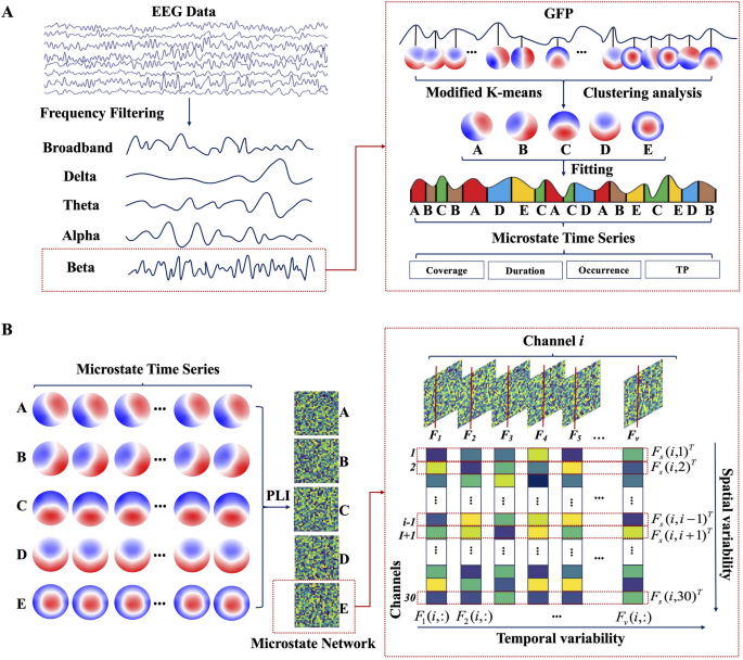
The scheme of the EEG microstate dynamics and spatiotemporal network analysis. A Steps for frequency–spectral microstate extraction, including bandpass filtering, global field power detection, microstate class identification, and microstate parameter analysis. B Steps for microstate-derived network analysis, including dynamic functional connectivity computation per microstate class by phase lag index, and quantification of temporal variability and spatial variability
EEG spectral microstate network analysis
The EEG microstate sequence for each individual was segmented into a series of discrete, non-overlapping intervals based on the assigned microstate labels (A-E). For each resulting microstate window, a functional connectivity network was constructed from 30 EEG electrodes using the Phase Lag Index (PLI). The PLI serves to measure the asymmetry level observed in the phase disparity between two signals [27]. Functional connectivity was estimated independently within each microstate segment, without concatenation or averaging across segments, resulting in a series of state-specific functional connectivity matrices. The segmentation algorithm adaptively defines the duration of each window, thereby avoiding arbitrary temporal partitioning and maintaining physiologically meaningful boundaries. Moreover, microstate segments, typically lasting between 60 and 300 ms, are considered quasi-stationary and have been empirically demonstrated to support reliable phase-based connectivity estimation [21]. Thus, the functional connectivity of paired EEG channels in the interval represented by the \(\:r\)-th microstate window was determined, as illustrated by formula (2),
$$ F_{r} \left( {i,j} \right) = \left| {~\left\langle {sign~\left[ {~sin\left( {\Delta \phi \left( {t_{l} } \right)} \right)~} \right]} \right\rangle ~} \right|l = 1,2,…,m_{r} ,i \ne j $$
(2)
where \(\:{F}_{r}(i,j)\) represents the functional connectivity between electrode channels \(\:i\) and \(\:j\) in the r-th microstate epoch. The notation \(\:\left\langle.\right\rangle\) is employed to denote the average value over that period. \(\:\Delta\varphi\:\left({t}_{l}\right)\) represents the phase differential determined at the \(\:l\)-th time instance, while \(\:{m}_{r}\) stands for the total number of time points within the \(\:r\)-th microstate epoch. By aggregating these PLI values for all pairs of EEG channels, the 30 × 30 adjacency matrix was constructed, which forms the brain network \(\:{F}_{r}\) for the \(\:r\)-th microstate window.
Subsequently, the functional connection networks corresponding to every distinct microstate category was divided into five different brain network sets (microstate networks A, B, C, D, and E). Utilizing these networks, the temporal and spatial variabilities were computed [21]. Temporal variability, by assessing the correlation between functional connectivity patterns of the same brain region across different time windows, captures the time-dependent changes of the functional architecture in specific brain areas, thereby providing insights into the temporal robustness of the region’s functional connectivity. The specific definition is shown in formula (3):
$$\:{T}_{i}=1-\frac{1}{v(v-1)}\sum\:_{p,q=1,p\ne\:q}^{v}\text{c}\text{o}\text{r}\text{r}\left({F}_{p}(i,:),{F}_{q}(i,:)\right)$$
(3)
where \(\:v\) is the number of microstate windows, \(\:{F}_{p}(i,:)\) indicates the functional arrangement of the \(\:i\)-th channel within the \(\:p\)-th microstate window, while \(\:corr({F}_{p}\left(i,:\right),{F}_{q}\left(i,:\right))\) calculates the correlation coefficient that measures the temporal similarity between two separate functional connectivity patterns. Spatial variability, by evaluating the correlation between the functional connectivity sequences of a particular brain region and those of other regions, reflects both the dynamic changes in local spatial functional connectivity and the spatial consistency of connectivity between regions. The definition is shown in formula (4),
$$\:{S}_{i}=1-\frac{1}{29\times\:28}\sum\:_{i,h=1,j\ne\:h\ne\:i}^{30}\text{c}\text{o}\text{r}\text{r}\left({F}_{s}(i,j),{F}_{s}(i,h)\right)$$
(4)
where \(\:corr({F}_{s}\left(i,j\right),{F}_{s}\left(i,h\right))\) denotes the correlation coefficient that quantifies the relationship between two different spatial functional connectivity patterns, \(\:{F}_{s}\left(i,j\right)\) and \(\:{F}_{s}\left(i,h\right)\). This metric is employed to assess the spatial consistency across all functional connectivity sequences associated with a particular scalp region (channel \(\:i\)) (Fig. 1B).
Clinical effect prediction
A feature set for classification was derived from microstate parameters, including coverage, duration, occurrence, and both temporal and spatial variability. These parameters were extracted across multiple frequency bands. To capture the spectral specificity of brain dynamics, these features were organized into distinct sets based on the following frequency bands: delta (1–4 Hz), theta (4–7 Hz), alpha (7–13 Hz), beta (13–30 Hz), and a broadband (1–30 Hz). A Random Forest classifier, implemented using a Bagging ensemble of decision trees, was trained for multi-class classification. To enhance model robustness and generalizability, hyperparameters (i.e., the number of trees, minimum leaf size, and maximum number of splits) were optimized via a Bayesian optimization algorithm. A nested cross-validation (CV) strategy was employed to prevent data leakage and overfitting. In this scheme, an inner 5-fold CV performed hyperparameter tuning, while an outer 5-fold CV provided an unbiased estimate of the model’s performance. To address potential class imbalance, class weights were set to be inversely proportional to class frequencies and applied during model training. The final model performance was determined by averaging the prediction metrics across the five outer folds of the nested CV. Classifier performance was comprehensively assessed using accuracy, sensitivity, and specificity. The results for each metric are reported as the mean ± standard deviation across these folds.
Statistical analysis
Data normality was evaluated by applying the Shapiro-Wilk test. The Mann-Whitney U test and independent t-tests were used to examine differences in demographic characteristics and clinical scores among the groups. Repeated measures Analysis of Variance was employed to evaluate group (PD-MCI, PD-NC, and HC) differences across narrowband and broadband microstate network metrics using four model specifications: (1) microstate parameters (3 groups × 3 parameters [coverage, duration, and occurrence] × 5 classes [MS-A, MS-B, MS-C, MS-D, and MS-E]), (2) transition probabilities (3 groups × 20 metrics [A to B/C/D/E, B to A/C/D/E, C to A/B/D/E, D to A/B/C/E, E to A/B/C/D]), (3) microstate network regional temporal or spatial variabilities (3 groups × 5 microstate levels × 30 channels), and (4) microstate network global temporal or spatial variabilities (3 groups × 5 classes [MS-A, MS-B, MS-C, MS-D, and MS-E]). Where significant main and interaction effects emerged (p < 0.05), post hoc analyses was conducted using Bonferroni-corrected paired-samples t-tests. Pearson correlations then quantified relationships between MoCA scores and group-discriminating features in PD subgroups (PD-MCI vs. PD-NC), with independent Bonferroni corrections applied to four metric families per frequency band: microstate parameters, transition probabilities, regional temporal or spatial variabilities, and global temporal or spatial variabilities.