We consider a system of N bosons in a two-dimensional isotropic harmonic potential, interacting with a force proportional to the square of the distance between the particles. The Hamiltonian of this system has the form11
$$begin{aligned} mathscr {H} = sum _{i=1}^Nleft[ -{hslash ^2over 2m}nabla ^{2}_{textbf{r}_{i}} + {m omega ^2textbf{r}^2_{i}over 2}+sum _{j=i+1}Lambda |textbf{r}_i-textbf{r}_j|^2right] , end{aligned}$$
(1)
which can be transformed into a dimensionless form using the spatial coordinates expressed in (sqrt{hslash /momega }), the interaction parameter (Lambda) in (m omega ^2) and the energy in (hslash / omega).
One-particle reduced density matrix
The integral representation of the one-particle reduced density matrix is as follows
$$begin{aligned} rho (textbf{r},textbf{r}^{‘})=int Psi ^{*}(textbf{r},textbf{r}_{2},…,textbf{r}_{N})Psi (textbf{r}^{‘},textbf{r}_{2},…,textbf{r}_{N})dtextbf{r}_{2}…dtextbf{r}_{N}. end{aligned}$$
(2)
Their eigenvectors (u_{k}(textbf{r})) (natural orbitals) and eigenvalues (lambda _{k}) (occupancies) are determined by the following integral eigenproblem
$$begin{aligned} int rho (textbf{r},textbf{r}^{‘})u_{k}(textbf{r}^{‘})dtextbf{r}^{‘}=lambda _{k}u_{k}(textbf{r}).end{aligned}$$
(3)
These eigenvalues can be interpreted as expansion coefficients in the Schmidt decomposition, while the corresponding eigenfunctions represent the natural orbitals of the system
$$begin{aligned} rho (textbf{r},textbf{r}^{‘})=sum _{k}lambda _{k}u^{*}_{k}(textbf{r}^{‘})u_{k}(textbf{r}).end{aligned}$$
(4)
The eigenvalues (lambda _{k}) are widely employed to quantify correlation effects in many-body systems and to distinguish between various quantum phases, including condensed and fragmented states. In the system under consideration, the one-particle reduced density matrix can be derived analytically in Cartesian coordinates19 and is conveniently expressed in polar coordinates as follows
$$begin{aligned} rho (textbf{r},textbf{r}^{‘})=A exp left( -{Bover 2}(r^2+{r^{‘}}^{2})+{Cover 2} r r^{‘}textrm{cos}(varphi -varphi ^{‘})right) , end{aligned}$$
(5)
with the normalization constant
$$begin{aligned} A=left( 2pi int _0^{infty } e^{-Br^2+frac{C}{2} r^2} r drright) ^{-1} = {omega over pi gamma }, end{aligned}$$
(6)
where
$$begin{aligned} B={omega over gamma }+{Cover 2}, C=left( {1-omega over N}right) ^2{(N-1)over gamma }, end{aligned}$$
(7)
and
$$begin{aligned} gamma ={(N-1+omega )over N}, omega =sqrt{1+2Lambda N}. end{aligned}$$
(8)
Diagonal representation of the one-particle reduced density matrix
The objective of this study is to derive the Schmidt decomposition of Eq. (5) in polar coordinates, providing a diagonal representation of the one-particle reduced density matrix. To this end, we first expand Eq. (5) in a Fourier-Lagrange series.
$$begin{aligned} rho (textbf{r},textbf{r}^{‘})={rho _{0}(r, r^{‘})over {2pi }}+sum _{l=1}{ rho _{l}(r,r^{‘}) textrm{cos}[l(varphi -varphi ^{‘})]over {pi }}, end{aligned}$$
(9)
where the l-partial wave component is given by the following integral
$$begin{aligned} rho _{l}(r, r^{‘})=int _{0}^{2pi } rho (textbf{r},textbf{r}^{‘}) textrm{cos}(ltheta ) dtheta ,end{aligned}$$
(10)
wherein (theta =varphi -varphi ^{‘}), which results in
$$begin{aligned} rho _{l}(r, r^{‘})=2Api exp left( -{Bover 2}(r^2+{r^{‘}}^2)right) I_{l}left( {C rr^{‘}over 2}right) ,end{aligned}$$
(11)
where we have employed an integral formula for the modified Bessel function of the first kind (I_{l}(z)), that is23
$$begin{aligned} int _{0}^{2pi }dtheta exp left( z cos (theta ) right) cos (l theta )=2pi I_{l}(z). end{aligned}$$
(12)
A detailed analysis indicates that the Schmidt decomposition of the l-partial component, denoted as (rho _{l}) in Eq. (11), can be derived by direct comparison with the Hardy-Hille formula24
$$begin{aligned} exp left( -{left( {1over 2}+{tover 1-t} right) (x+y)} right) I_{alpha }left( {2 sqrt{ xyt}over 1-t}right) = sum _{n=0} {n! t^{n+frac{alpha }{2}}(1-t)over (n+alpha )!}(xy)^{frac{alpha }{2}}exp left( -{(x+y)over 2} right) L_{n}^alpha (x)L_{n}^{alpha }(y), end{aligned}$$
(13)
where (L_{n}^{alpha }(x)) is the generalized Laguerre polynonomial and
$$begin{aligned} t=-1+{4Bover C^2}left( 2B-sqrt{4B^2-C^2}right) . end{aligned}$$
(14)
By substituting (x = z^2r^2) and (y = z^2{r^{‘}}^2) into the formula (13), where
$$begin{aligned} z={(4B^2-C^2)^{1over 4}over sqrt{2}},end{aligned}$$
(15)
we derive the matching condition
$$begin{aligned} B=left( 1 + 2t(1 – t)^{-1}right) z^2, C=4sqrt{t}(1 – t)^{-1}z^2,end{aligned}$$
(16)
which, together with the requirement that Schmidt orbitals be normalized, yields
$$begin{aligned} rho _{l}(r,r^{‘})=sum _{n} lambda _{n,l}v_{n,l}(r^{‘}) v_{n,l}(r),end{aligned}$$
(17)
with
$$begin{aligned} v_{nl}(r)=sqrt{{2 n! z^2 over (n+|l|)!}}(z r)^{|l|}e^{-z^2r^2/2}L_{n}^{|l|}(z^2 r^2), end{aligned}$$
(18)
and
$$begin{aligned} lambda _{nl}={Api t^{M}(1-t)over z^{2}}, qquad text {with} qquad M=n+frac{|l|}{2}.end{aligned}$$
(19)
Using the above expressions and the identity (cos (ltheta ) = (exp (i ltheta ) + exp (-i ltheta ))/2), where i is an imaginary unit, we can represent the 1-RDM as follows
$$begin{aligned} rho (textbf{r},textbf{r}^{‘})=sum _{n=0}^{infty } sum _{l=-infty }^{infty } lambda _{n,l}u^{*}_{n,l}(textbf{r}^{‘})u_{n,l}(textbf{r}), end{aligned}$$
(20)
where
$$begin{aligned} u^{}_{n,l}(textbf{r})={v_{n,l}(r)}{e^{i lvarphi }over sqrt{2pi }}. end{aligned}$$
(21)
The orbitals (21) form an orthonormal basis set
$$begin{aligned} int _{0}^{2pi } int _{0}^{infty }dvarphi dr [r u^{*}_{n,l}(textbf{r})u^{}_{n^{‘}l^{‘}}(textbf{r})]=delta _{nn^{‘}}delta _{ll^{‘}},end{aligned}$$
(22)
and they can be recognized as the natural orbitals of the occupancies (19). The values of (lambda _{n,l}) are ((2M+1))-fold degenerate indicating that for given M, there exist exactly ((2M+1)) orthogonal orbitals corresponding to (lambda _{n,l}). We note that while the Schmidt decomposition uniquely determines the set of non-zero occupation numbers, the decomposition is not unique. Alternative forms of Schmidt orbitals can be constructed for the degenerate points (lambda _{n,l} = lambda _{n|l|}) as follows25,26
$$begin{aligned} chi _{n,l}(textbf{r})= {left{ begin{array}{ll} frac{1}{sqrt{2}} (u_{n,-l}(textbf{r})+u_{n,l}(textbf{r})), & text {for} lne 0\ \ u_{n,0}(textbf{r}), & text {for} l=0 end{array}right. } qquad qquad xi _{n,l}(textbf{r}) = {left{ begin{array}{ll} frac{i}{sqrt{2}}(u_{n,-l}(textbf{r})-u_{n,l}(textbf{r})) , & text {for} lne 0\ \ 0, & text {for} l=0 end{array}right. }. end{aligned}$$
(23)
The family ({chi _{n,l}, xi _{n,l}}) forms a complete and orthonormal set. In terms of the orbitals (23), the 1-RDM takes the form
$$begin{aligned} rho (textbf{r},textbf{r}^{‘})=sum _{l,n=0}^{infty } lambda _{n,l} left( chi _{n,l}(textbf{r})chi _{n,l}(mathbf {r’})+xi _{n,l}(textbf{r})xi _{n,l}(mathbf {r’})right) . end{aligned}$$
(24)
Collective occupancies, participation, and correlation
There are many different quantities for studying the properties of many-body states. In the case of isotropic symmetry, one of them is the collective occupancy, defined as the sum of occupancies with angular momentum l27
$$begin{aligned} eta _l= sum _n lambda _{n,l}=frac{n_{l}}{N}, end{aligned}$$
(25)
where (n_{l}) denotes the number of particles with that angular momentum. This quantity determines a fraction of particles with a given l. For the present system, the collective occupancy is given by the geometric series ((0< t < 1)) and can thus be accurately determined in closed analytical form
$$begin{aligned} eta _l= frac{ pi A t^{frac{|l|}{2}}}{z^2}, end{aligned}$$
(26)
which gives us a unique opportunity to examine its behavior in the full interaction regime and the general case of N particles. Another closely related quantity is participation, defined as
$$begin{aligned} K_{eta }= left( sum _{l} eta _l^2 right) ^{-1},end{aligned}$$
(27)
which measures the effective number of collective occupancies, i.e., the number of l fragments that contribute significantly. The collective occupancies and this tool offer insight into correlations in the single-particle angular momentum domain. For the same reason as for collective occupancy, this measure can be obtained analytically.
$$begin{aligned} K_{eta }=frac{z^4(1-t)}{pi ^2 A^2 (1+t)}.end{aligned}$$
(28)
By contrast, participation
$$begin{aligned} K=left( sum _{n,l} lambda _{n,l}^2 right) ^{-1} =frac{z^4}{pi ^2 A^2} end{aligned}$$
(29)
quantifies the effective number of natural orbitals and serves as an indicator of the degree of single-particle correlations28. More specifically, it assesses how a subsystem containing one particle correlates with a subsystem composed of the remaining particles.
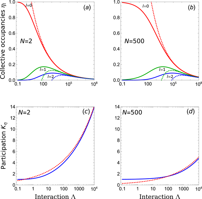
Graphs (a) and (b) show the behaviors of collective occupancies as functions of interaction strength (Lambda) for two different particle numbers (N=2) and (N=500), respectively. The dashed lines represent the approximation results (30). The strength of the interaction (Lambda) is expressed in units of (m omega ^2). The graphs (c) and (d) illustrate the corresponding results for the participation (K_{eta }), together with its approximation obtained from the expansion to infinity, (Lambda rightarrow infty): (K_{eta } approx 2beta ^{-1}(N)Lambda ^{1/4}) (dashed lines).