A fluorescent-protein spin qubit | Nature

Protein expression and purification

In Figs. 1–4 and 5d, we measured EYFP with the mutations S2insL/S65G/V68L/S72A/T203Y/H231L of avGFP, with an additional 6x His tag on the N-terminus (the full amino acid sequence is given at the end of this section). The protein was expressed using a pET vector constructed using HiFi assembly from Addgene plasmids 78466 and 29653. The resulting vector was sequenced to confirm the inclusion of the EYFP gene. The plasmid was transformed into BL21 (DE3) E. coli for protein expression. Single colonies of the cells were picked from a kanamycin plate and incubated in 5 ml LB medium at 37 °C, 250 RPM overnight. Cultures were transferred into a 2-l flask with 500 ml LB medium and continued incubating at 37 °C. Once the optical density at 600 nm D₆₀₀ reached about 0.6, protein expression was induced with isopropyl β-D-1-thiogalactopyranoside and the temperature was lowered to 30 °C. Cells were pelleted after 16 h and lysed using 4 ml B-PER (Thermo Scientific) per gram of cells. The supernatant pre- and post-lysis appeared yellow and was loaded onto a Ni-NTA spin column (Thermo Scientific) and washed 3 times using 10 ml solution containing 50 mM sodium phosphate buffer, 500 mM NaCl and 25 mM imidazole. Elution buffer (50 mM sodium phosphate buffer, 500 mM NaCl and 250 mM imidazole) was used to elute the purified protein from the column. Buffer exchange using a 3-kDa molecular weight cut-off ultracentrifugal unit suspended the protein in the sample buffer (50 mM tris, 150 mM NaCl, 2 mM EDTA). The protein solution was concentrated, estimated to be 6 mM by measuring the optical density of the samples at 515 nm, and stored at −80 °C. When measured at cryogenic temperatures, the protein solution was mixed with 20% v/v DMSO.

The following is the amino acid sequence of the EYFP we measured from E. coli: MGSSHHHHHHENLYFQSNIMLSKGEELFTGVVPILVELDGDVNGHKFSVSGEGEGDATYGKLTLKFICTTGKLPVPWPTLVTTFGYGLQCFARYPDHMKQHDFFKSAMPEGYVQERTIFFKDDGNYKTRAEVKFEGDTLVNRIELKGIDFKEDGNILGHKLEYNYNSHNVYIMADKQKNGIKVNFKIRHNIEDGSVQLADHYQQNTPIGDGPVLLPDNHYLSYQSALSKDPNEKRDHMVLLEFVTAAGITLGMDELYKSTGSG*.

Preparation for ODMR of bacteria cells at room temperature

EYFP was expressed in E. coli as discussed above. The E. coli were pelleted, the supernatant was replaced by sample buffer (50 mM tris, 150 mM NaCl, 2 mM EDTA) and the pellet was stored at −20 °C. The sample was subsequently thawed at room temperature, loose cell debris and supernatant were discarded, and a sample of cells was scraped onto a 0.17-mm coverslip. The coverslip was placed on a printed circuit board and immediately measured using an oil immersion objective with 1.3 numerical aperture.

EYFP expression in mammalian cells

The plasmid pNWA171 encodes a second-generation chimeric antigen receptor (CAR) targeting CD19. The vector and a gene fragment encoding EYFP (Twist Bioscience) were both digested with MulI and SbfI restriction enzymes and then ligated with T4 ligase. The resulting plasmid was sequenced to confirm the inclusion of the EYFP gene and the deletion of the CAR19 gene. The plasmid was maxi-prepped, transfected with the Lenti-X 293T cell line (Takara Bio) with PEI max (Polysciences), and then cultured for 48 h for EYFP production. On the day of the experiment, a coverslip with photolithographically patterned waveguides was sterilized using 70% isopropanol, washed extensively with PBS and then incubated with 0.01% poly-l-lysine (MilliporeSigma) solution for 5 min. The residual poly-lysine solution was washed extensively with PBS. Cells were dissociated from the culture flask with trypLE (Gibco, Thermo Fisher Scientific) and then resuspended in DMEM supplemented with 10% HIFBS with a cell density of 1 × 10⁷ cells per ml. Finally, the cell suspension was incubated on the coverslip under 37 °C, 5% CO₂ for 3 h. The coverslip was gently washed with PBS, allowing only the adherent cells to remain for the experiments in Fig. 5a–c. The cells were then imaged in PBS.

The following is the amino acid sequence of the EYFP expressed in mammalian cells: MLSKGEELFTGVVPILVELDGDVNGHKFSVSGEGEGDATYGKLTLKFICTTGKLPVPWPTLVTTFGYGLQCFARYPDHMKQHDFFKSAMPEGYVQERTIFFKDDGNYKTRAEVKFEGDTLVNRIELKGIDFKEDGNILGHKLEYNYNSHNVYIMADKQKNGIKVNFKIRHNIEDGSVQLADHYQQNTPIGDGPVLLPDNHYLSYQSALSKDPNEKRDHMVLLEFVTAAGITLGMDELYK*.

Experimental methods

Experiments were performed in a closed-cycle liquid-helium cryostat with temperature control from 4 K to room temperature using a custom confocal microscope (Extended Data Fig. 2). Prolonged exposure to laser excitation results in photobleaching of the EYFP (Extended Data Fig. 4c). To counteract photobleaching, the microscope was scanned over the area within a single photolithographically patterned loop structure, except for the low temperature Rabi (Fig. 3a) and room temperature data (Figs. 4 and 5d), where it was at a fixed location. Digital signals to pulse the lasers and microwave tones for driving the spin transitions were generated using the Real Digital RFSoC 4×2 running the QICK platform⁶³ with a custom version of the software and firmware designed for optically addressable spin qubits. In Fig. 5, the wide-field fluorescence image was captured using a Leica DMi8 microscope.

Data analysis

OADF photon counts were integrated over the first approximately 300 ns following the rising edge of the 912-nm laser pulse and over multiple experiments. The contrast in Figs. 1d, 2a,c, 3a and 4a,b, and Extended Data Figs. 7b, 8, and 12b,c are defined by the following normalization C = [PL_sig(ω) − PL_back(ω)]/PL_back(ω), where PL_sig(ω) refers to the photoluminescence with microwave output switched on and PL_back(ω) refers to the photoluminescence with microwave output switched off. The contrast in Fig. 3b,c is defined as (C=frac{{rm{PL}}(theta =-{rm{pi }}/2)-{rm{PL}}(theta =+{rm{pi }}/2)}{{rm{PL}}(theta =-{rm{pi }}/2)+{rm{PL}}(theta =+{rm{pi }}/2)}) normalized to the fit maximum, where PL(θ) corresponds to the photoluminescence signal with the last microwave pulse having rotation angle θ. Finally, the contrast in Fig. 3d is defined as C = [PL(θ = π) − PL(θ = 0)]/PL(θ = 0). All stated errors are one standard deviation.

Sample degradation

The conformational stability of EYFP was interrogated using circular dichroism spectroscopy. The EYFP sample prepared at 100 μM in storage buffer (50 mM Tris, 150 mM NaCl and 2 mM EDTA; pH 7.4) was measured hours after purification and another sample of the same concentration was measured after cooling to 80 K in our cryostat at 5 mM concentration with 20% DMSO. Circular dichroism spectra between 180 nm and 260 nm at a scan speed of 100 nm min⁻¹ and bandwidth of 5 nm were taken using a Jasco J-1500 spectropolarimeter. Extended Data Fig. 4a shows the resulting data after averaging over three scans. The spectra show a minimum at 230 nm, indicating that the main secondary structure content of EYFP is a β-sheet configuration. No substantial differences were observed between the spectra of the two samples, suggesting that the cool-down and warm-up processes used in the experiments did not alter the structure of EYFP.

Computational methods

The orbital structures in Fig. 1c are the result of TDDFT^64,65 calculations on the negatively charged model of the EYFP fluorophore terminated with methyl groups. The geometry was optimized using the conductor-like polarizable continuum model⁶⁶ with a dielectric constant ε = 4 to mimic the protein environment. The ground-state geometry optimizations for the singlet (S0) and triplet (T1) states were performed using the Gaussian 16⁶⁷ package at B3LYP/def2-TZVP level. The ORCA 5.4.0 package⁶⁸ was used for the TDDFT calculations to compute the vertical excitation energies. Range-separated hybrid functionals CAM-B3LYP⁶⁹ and ωB97X-D3⁷⁰ were used with the B3LYP/def2-TZVP/ε = 4 optimized geometries and def2-QZVPP basis sets for the TDDFT calculations. The zero-field splitting calculations for the D and E parameters were performed at the T1 optimized geometry with a series of functionals shown in Extended Data Fig. 6. The absolute D and E parameters were calculated using spin–orbit coupling treated at the spin–orbit mean-field theory (as implemented in ORCA 5.4.0 package). The coupled-perturbed method was used for calculating the zero-field splitting tensor with DFT⁷¹.

TDDFT calculations

TDDFT calculations predict the first bright singlet–singlet excitation to occur from the highest occupied molecular orbital (HOMO) to the lowest unoccupied molecular orbital (LUMO), showcasing a π → π* nature of the transition. This S0 → S1 transition corresponds to the experimental absorption at 2.54 eV. Both CAM-B3LYP and ωB97X-D3 predict an energy gap of about 3.02 eV between the S1 and S0 states. The results overestimate the experimental value, similar to an earlier report for gas-phase calculations⁷². The first bright excitation using the triplet optimized geometry occurs for T1 → T2, which also corresponds to a π → π* transition. Although this vertical excitation energy of 1.49 eV also overestimates the experimentally observed triplet–triplet absorption at 1.37 eV, it characterizes the T1 → T2 transition to involve a singly occupied molecular orbital (SOMO), where the electron is excited from SOMO-2 to SOMO-1. The oscillator strengths and transition characters for all the transitions are reported in Supplementary Tables 1–4.

Simulation of magnetic resonance spectrum

Solving for the eigenvalues of the Hamiltonian from equation (1) provides the T_x–T_z, T_y–T_z and T_x–T_y transition frequencies as a function of the magnetic field (B). Importantly the transition frequencies depend not only on the field strength but also on the molecule’s orientation relative to the magnetic field. Assuming that the EYFP molecules are randomly oriented, we sample 10,000 uniformly distributed orientations. To simulate the ODMR spectra in Fig. 2b,c, we incorporate the single-molecule ODMR linewidth (γ). The resonance for a single EYFP molecule is then modelled by a Lorentzian of the form (L(omega )=frac{{a}_{x-z}}{1+{left(frac{omega -{omega }_{x-{rm{z}}}}{gamma }right)}^{2}}+frac{{a}_{y-z}}{1+{left(frac{omega -{omega }_{y-z}}{gamma }right)}^{2}},) where a_x−z and a_y−z denote the ODMR contrast, and ω_x–z and ω_y–z denote the transition frequencies for the T_x–T_z and the T_y–T_z transitions, respectively. It is noted that our model simplifies the fitting by only considering the T_x–T_z and T_y–T_z resonance while omitting the T_x–T_y transition, which has a reduced ODMR contrast and experimental data that overlap with a harmonic of our signal generator. We iteratively optimize the fit parameters D, E, a_x−z, a_y−z and γ by minimizing the cost function (C={sum }_{i}{(n({omega }_{i})-L({omega }_{i}))}^{2}), where (n({omega }_{i})) denotes the experimentally observed ODMR spectra at the following fields: 2.1 mT, 4.5 mT, 6.1 mT, 8.2 mT and 10 mT. We find D = (2π) × (2.356 ± 0.004) GHz, E = (2π) × (0.458 ± 0.003) GHz, a_x−z = (0.17 ± 0.02), a_y−z = (0.129 ± 0.008) and γ = (2π) × (33 ± 4) MHz.

Rabi simulation

We computationally investigated the origin of the Rabi decay shown in Fig. 3a. Interestingly, we observed that the decay time increases with decreasing microwave power (Extended Data Fig. 7b) suggesting that loss in Rabi signal is not caused by dephasing. We simulated inhomogeneous broadening by sampling over a Gaussian distribution with a (2π) × 33 MHz standard deviation. The Rabi frequency depends on the molecule orientation with respect to the microwave drive field resulting in a fast decay that qualitatively captures our experimental observations (Extended Data Fig. 7c; a histogram of the Rabi frequencies is shown in the inset). In addition, the simulation captures the experimental behaviour that the decay time increases with decreasing microwave power (Extended Data Fig. 7d). We note that the inhomogeneous Rabi drive cannot be explained by spatial gradients caused by the loop geometry (Extended Data Fig. 7a).

Estimation of number of measured molecules

Knife-edge measurements of the 488-nm laser spot (Extended Data Fig. 9) estimate a beam waist w₀ = 2.81 μm (the larger between x, y) and Rayleigh range z_R = 13.18 μm. We assume a Gaussian beam with intensity (I(r,z)={I}_{0}{left(frac{{w}_{0}}{w(z)}right)}^{2}{{rm{e}}}^{frac{-2{r}^{2}}{w{(z)}^{2}}}), where (w(z)={w}_{0}sqrt{1+{left(frac{z}{{z}_{{rm{R}}}}right)}^{2}}) and r is the radial distance, z is the distance from focus and I₀ is the maximum intensity. We also assume that the collection and 488-nm excitation beam have the same point spread function, resulting in a confocal volume (V={int }_{-infty }^{infty }{int }_{0}^{2{rm{pi }}}{int }_{0}^{infty }{left(frac{1}{{I}_{0}}I(r,z)right)}^{2}r,{rm{d}}r,{rm{d}}phi ,{rm{d}}z={z}_{{rm{R}}}{({rm{pi }}{w}_{0})}^{2}/4). Using this volume and a sample concentration of 5 mM, we find that the effective number of molecules in our excitation volume is 773 × 10⁶ molecules. We note that this estimate serves as an upper limit, as we collect into a single-mode fibre, but our imaging system is not diffraction limited due to poor alignment through the cryostat window and sapphire sample coverslip. With diffraction-limited imaging, we estimate that we would measure about 810-times-fewer molecules with approximately the same brightness, providing about 28-times-better sensitivity than in this work.

Sensitivity estimation

The minimum signal that can be detected when integrating for a duration T is given by S_T/σ_T = 1, where S_T denotes the signal and σ_T denotes the standard deviation of S_T. In the following, the system’s response is linear with respect to a small field (δB) such that (frac{{rm{d}}{S}_{T}/{rm{d}}Btimes {delta }B}{{sigma }_{T}}=1). Therefore, the minimum field that can be detected is

where (frac{{rm{d}}{S}_{T}}{{rm{d}}B}) is maximized. Assuming the measurement is shot-noise limited, the sensitivity is (eta ={{delta }B}_{min }sqrt{T}) (ref. ²).

It is noted that we report two sensitivities: first, the experimentally measured sensitivity for an ensemble of 773 × 10⁶ molecules, which has units of T Hz^−1/2. Second, we normalize the sensitivity to the total number of qubits measured in units of mol, which has units of T mol^1/2 Hz^−1/2.

DC sensitivity (293 K)

To quantify the DC field sensitivity, we measure the difference of the photoluminescence at ω_a = (2π) × 3.54 GHz and ω_b = (2π) × 3.43 GHz, and normalize the signal to the photoluminescence in the absence of microwaves (PL_back). The resulting signal measured over T = 15 min is then given by C_T = [PL_sig(ω_a) − PL_sig(ω_b)/PL_back]. The fit has a slope of dS_T/dB₀ = 5.0 T⁻¹ and the residuals (Extended Data Fig. 10a) have a standard deviation σ_T = 4.6 × 10⁻⁴ yielding a sensitivity of (eta =frac{{sigma }_{T}}{{rm{d}}{S}_{T}/{rm{d}}B}sqrt{T}=2.7,{rm{m}}{rm{T}},{{rm{H}}{rm{z}}}^{-1/2}). Assuming an excitation volume of 256 μm³ and an EYFP concentration of 5 mM, which translates into 773 × 10⁶ molecules, we find a room-temperature DC magnetic-field sensitivity of (2.7frac{{rm{mT}}}{sqrt{{rm{Hz}}}}sqrt{frac{773times {10}^{6}}{6.022times {10}^{23}frac{1}{{rm{mol}}}}}=98,{rm{pT}},{{rm{mol}}}^{1/2},{{rm{Hz}}}^{-1/2}).

AC sensitivity (80 K)

AC sensing of small fields can be done using the CPMG sequence shown in Extended Data Fig. 10b. The signal of a single CPMG sequence is then given by ({S}_{pm }=frac{{n}_{Delta }}{2}(1pm sin (phi ))+frac{{n}_{Sigma }}{2}), where n_Δ denotes the difference in photon count between the T_x and T_z state, n_Σ their average, and the sign denotes the phase of the last π/2-pulse. Assuming a sinusoidal magnetic field with amplitude δB_AC, frequency T_CPMG/(2N) and in phase with the CPMG sequence, we can write the accumulated phase as (phi ={gamma }_{{rm{eff}}}delta {B}_{{rm{AC}}}{T}_{{rm{CPMG}}}W), with W = 2/π. The detected signal is then given by (S={S}_{+}-{S}_{-}={n}_{Delta },sin (2{gamma }_{{rm{eff}}}delta {B}_{{rm{AC}}}{T}_{{rm{CPMG}}}/{rm{pi }})) and the sensitivity by (eta =frac{{rm{pi }}}{2({n}_{Delta }/{{sigma }}_{n}){|gamma }_{{rm{e}}{rm{f}}{rm{f}}},|,{T}_{{rm{C}}{rm{P}}{rm{M}}{rm{G}}}}sqrt{2({T}_{{rm{C}}{rm{P}}{rm{M}}{rm{G}}}+{T}_{0})}), where σ_n denotes the standard deviation of n_Δ and T₀ is the experimental overhead time. The factor (sqrt{2}) originates from measuring n_Δ with two CPMG sequences. To experimentally estimate the AC sensitivity of EYFP, we integrated the signal over 250,000 experiments. We fit the difference in photon counts n_Δ,250,000 = 4,541 × exp(−(T_CPMG/5.35 μs)²) as a function of T_CPMG (Extended Data Fig. 10c) and σ_n,250,000 = 288 from the corresponding residual (Extended Data Fig. 10d). We can now estimate for a single experiment that ({n}_{Delta }=frac{{n}_{Delta ,mathrm{250,000}}}{mathrm{250,000}}) and ({{sigma }}_{n}=frac{{{sigma }}_{n,mathrm{250,000}}}{sqrt{mathrm{250,000}}}). Under these conditions, we find T_CPMG = 3.68 μs to be the optimal sensing duration (Extended Data Fig. 10e). Assuming an effective gyromagnetic ratio of ({gamma }_{{rm{e}}{rm{f}}{rm{f}}}=(2{rm{pi }})times -7.63,{rm{G}}{rm{H}}{rm{z}},{{rm{T}}}^{-1}) (that is, operating at B = 4.65 mT) and using T₀ = 60 μs, this results in a field sensitivity of η = 5.11 μT Hz^−1/2. Given that we measured approximately 773 × 10⁶ molecules, this translates into a sensitivity of (5.11frac{{rm{mu }}{rm{T}}}{sqrt{{rm{Hz}}}}sqrt{frac{773times {10}^{6}}{6.022times {10}^{23}frac{1}{{rm{mol}}}}}=183,{rm{fT}},{{rm{mol}}}^{1/2},{{rm{Hz}}}^{-1/2}).

NMR sensing limit of detection

In this section, we consider a thought experiment where we calculate the sensitivity of an ensemble of N fusion proteins, each consisting of a EYFP protein conjugated to a target protein that contains a single ¹⁹F nuclear spin. This ¹⁹F nuclear spin is separated by 5 nm from the qubit and produces a local magnetic field of δB = 18 nT at the location of the fluorophore. The field strength δB is dominated by the target ¹⁹F spin in the fusion proteins, as other ¹⁹F spins are significantly farther away and do not contribute to the signal. Starting from the AC sensitivity calculation (eta =frac{{rm{pi }}}{2({n}_{Delta }/{{sigma }}_{n}),|,{gamma }_{{rm{e}}{rm{f}}{rm{f}}},|,{T}_{{rm{C}}{rm{P}}{rm{M}}{rm{G}}}}sqrt{2({T}_{{rm{C}}{rm{P}}{rm{M}}{rm{G}}}+{T}_{0})}), we derive the limit of detection for NMR spectroscopy. However, in NMR only a small fraction of nuclear spins are polarized. Using the nuclear spin polarization (p), the overall signal is reduced to (S=p{n}_{Delta },sin (2{gamma }_{{rm{e}}{rm{f}}{rm{f}}}delta {B}_{{rm{A}}{rm{C}}}{T}_{{rm{C}}{rm{P}}{rm{M}}{rm{G}}}/{rm{pi }})), resulting in a sensitivity of ({eta }_{p}=frac{{rm{pi }}}{2(p{n}_{Delta }/{{sigma }}_{n}),|,{gamma }_{{rm{e}}{rm{f}}{rm{f}}},|,{T}_{{rm{C}}{rm{P}}{rm{M}}{rm{G}}}}sqrt{2({T}_{{rm{C}}{rm{P}}{rm{M}}{rm{G}}}+{T}_{0})}=frac{1}{p}eta ). This results in a polarization-adjusted sensitivity of ({eta }_{p}=frac{1}{p}183,{rm{fT}},{{rm{mol}}}^{1/2},{{rm{Hz}}}^{-1/2}) (see main text), allowing us to detect a magnetic field of ({delta }B=frac{1}{sqrt{N}sqrt{T}},{eta }_{p}). Solving for N we find a limit of detection of (N=frac{1}{T}{left({eta }_{p}frac{1}{{delta }B}right)}^{2}=frac{1}{T}frac{94}{p},{rm{pmol}},{{rm{Hz}}}^{-1}).

Improved optical readout

We estimate the improvements that will be gained with future advances in the optical readout of EYFP. For comparison purposes, ref. ¹³ collected 0.02 photons from a single nitrogen-vacancy centre per experiment cycle. In Extended Data Fig. 10c, we measure 0.167 photons per experiment cycle from an ensemble of 773 × 10⁶ EYFP molecules, which corresponds to 2.2 × 10⁻¹⁰ photons per molecule per experiment cycle. This means that in our experiment, we collect approximately 10⁻⁸-times-fewer photons from an EYFP molecule compared with a nitrogen-vacancy centre.

OADF readout yields at most one photon per molecule per experiment cycle. This can, in principle, be improved by utilizing the cycling transition in the singlet manifold. Such a cycling could be accomplished by applying a short 912-nm pulse that transfers only the short-lived triplet states (T_x,y) into the singlet ground state but not the long-lived triplet state (T_z). The singlet population could then be probed by a subsequent 488-nm laser pulse. It is noted that this approach, relying on fluorescence cycling of the singlet state, would require an efficient triplet initialization since the population that remains in the singlet ground state after initialization would contribute a background signal to the readout.

Although we have not yet quantified the shelving efficiency, it is probably low in the current experimental configuration. Improvements in shelving efficiency translate directly into gains in signal. Let us assume an ideal scenario where we achieve 100% shelving efficiency during the 488-nm initialization laser pulse. This implies that all molecules are in the T1 state following initialization and contribute to our sensing experiment. If the shelving efficiency increases from ζ₀ to 100%, then the number of probed molecules, and thus the photon number, also increases by 1/ζ₀. The T1 triplet yield is approximately 0.003 (refs. ^39,40), so by utilizing fluorescence readout, this would yield a signal amplification of 333 due to the improved cyclicity. Improved triplet shelving efficiency also allows for a much shorter initialization laser pulse. In saturation, the EYFP should shelve in approximately 333 × 3 ns = 1 μs. The readout laser pulse can also be shortened to about 1 μs. This yields an improvement of (frac{30,{rm{mu }}{rm{s}}+30,{rm{mu }}{rm{s}}}{1,{rm{mu }}{rm{s}}+1,{rm{mu }}{rm{s}}}=30). Use of an oil immersion objective with a modest numerical aperture of 1.3 would yield a (1.3/0.7)² = 3.4 improvement in photon counts. As discussed in the section above, reduced aberrations would result in an 810-times improvement in signal.

Combining all of these improvements yields an enhancement of (1/{zeta }_{0}times 2.75times {10}^{7}) signal photons, which should allow us to meet or exceed the sensitivity of a single nitrogen-vacancy centre.

Room temperature ODMR mechanism

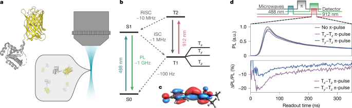
At room temperature, we observe an ODMR signal that originates from a different mechanism than at low temperatures. The 488-nm laser pulse initializes the EYFP into its triplet state and polarizes its triplet spin sublevels. This spin polarization is quickly eliminated by fast spin-lattice relaxation within 100 ns. Consequently, ODMR at room temperature is not observable using the same pulse sequence we used at 80 K where the microwave pulse is delayed from the spin readout by at least 100 ns (Extended Data Fig. 12c). Nevertheless, ODMR measurements are obtained at room temperature despite equilibration of the spin levels after the 488-nm laser pulse. As long as the EYFP persists in the triplet state, it can be re-excited to the higher-lying triplet, T2, using the 912-nm laser. Because the T_x and T_y spin sublevels undergo RISC to the singlet manifold much faster than the T_z sublevel, the 912-nm laser causes the triplet manifold to regain a spin polarization by depopulating the T_x and T_y sublevels. ODMR contrast can then be observed when a subsequent microwave drive is resonant with the T_x–T_z or T_y–T_z transitions transferring population from T_z back into T_x or T_y (Extended Data Fig. 12b).