Dataset
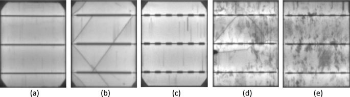
The researchers introduced a publicly available dataset of solar cell images26, comprising high-resolution electroluminescence (EL) captures from both monocrystalline and polycrystalline photovoltaic modules60. Each solar cell image has a resolution of 2624 pixels (300 × 300). The dataset comprises images collected from 44 distinct PV modules (18 monocrystalline and 26 polycrystalline types). The PV module images were captured under controlled conditions at the production facility to minimize detrimental effects like overexposure. These controlled settings were necessary as background irradiation could dominate EL irradiation. Imaging in a dark room ensured even lighting, with only the PV module generating light. For classification purposes, the extracted cells were randomly presented to experts familiar with various flaws in EL images. These experts focused on known faults causing more than 3% power loss from initial output, following principles summarized in16. The experts evaluated: (1) whether the cell was functional or faulty, and (2) their confidence in this assessment. The confident assessors’ evaluations were used directly as labels. For less confident assessors, all cells (both functional and defective) were labeled as defective but with different weights: 33% weight for uncertain functional cell ratings and 67% weight for uncertain defective cell ratings. Table 2 shows the evaluators’ ratings and corresponding labels and weights.
Table 3 displays the distribution of labeled solar cells by PV module type. The dataset was split with 25% (656 cells) for testing and 75% (1968 cells) for training. Stratified sampling maintained the class distribution in both sets. The dataset consists of eight classes: four representing defect percentages (0%, 33%, 66%, and 100%) and four representing solar cell types (monocrystalline or polycrystalline) for each defect percentage.
Preprocessing and data augmentation
Large datasets are crucial for optimizing deep learning model performance and preventing overfitting. While increasing dataset size generally enhances model accuracy, practical constraints often necessitate data augmentation techniques such as cropping, rotation, noise injection, and image inversion50,60. In this study, limited training data prompted dataset expansion through offline augmentation methods. These techniques proved particularly suitable for EL image analysis since defect orientation does not impact classification outcomes in solar cell fault detection. The research team developed a novel GAN-based augmentation framework comprising:
-
1.
A generative network (G-network) with:
-
2.
A discriminative network (D-network) for adversarial training (as illustrated in Fig. 2)
The D-network consists of 4 convolutional layers and a fully connected layer that determines whether an image is real or fake. Table 3 lists the parameters for both network structures. The proposed model uses a G-network that takes noise as input and produces fake images as output. The D-network then distinguishes between generated and real images. The Earth Mover (EM) distance measures the difference between generated and real images, with cost functions for the G-network and D-network defined by Eqs. (1) and (2).
$${G}_{loss}=-{E}_{x}- {p}_{g}[ {f}_{w}left(xright) ]$$
(1)
$${D}_{loss}=-{E}_{x}- {p}_{g}left[ {f}_{w}left(xright) right]-{E}_{x}-{p}_{r}left[ {f}_{w}left(xright)right]$$
(2)
({text{f}}_{text{w}}left(text{x}right)) where symbolizes the D-network model, with input x coming from either generated or actual pictures. RMS prop (Root Mean Square Prop) was selected as the optimization technique for training the model; ({D}_{loss}) should be minimized to approximate the Wasserstein distance; the initial hyperparameters of GAN are exposed in Table 5. Matched with traditional image processing methods, GAN-based image processing requires more computational time and has moderately high demand on computer hardware. EL images of dissimilar defects generated using the GAN model are shown in Fig. 2. This method has advantages over the data enhancement method: GAN can generate new images, GAN can extract deep picture characteristics for image improvement, and GAN can be used to enhance the image of defects.
The enhanced images generated through this process exhibit substantial qualitative improvements that can potentially enhance CNN model performance during training. However, several critical considerations must be addressed: (1) training dataset size must be carefully optimized to prevent overfitting, and (2) the inherent stochasticity of GAN-based image generation requires particular attention. To address data scarcity challenges, we implement a two-stage augmentation pipeline where the GAN model first generates synthetic samples, which are then combined with the original dataset for subsequent CNN training. This hybrid approach significantly improves augmentation efficiency in data-limited scenarios. In our study, we implemented a GAN-based oversampling strategy referred to as AUG300, in which 300 synthetic images were generated per class, regardless of the original class balance. Unlike traditional methods such as SMOTE, which operate in feature space using interpolation between existing samples, our approach leverages the ability of GANs to generate entirely new, high-resolution electroluminescence images with realistic defect patterns. This strategy not only enhances the diversity of the dataset but also introduces a controlled augmentation volume that helps counteract class imbalance and model bias. By enriching all classes equally and consistently, AUG300 contributed to improving classification robustness and generalization in our deep learning models.(Table 4).
To ensure the physical realism and class-specific consistency of the GAN-generated EL images, multiple validation steps were performed. A visual inspection was conducted by comparing synthetic images with real EL samples, highlighting their similarity in crack structures, brightness levels, and texture patterns. As illustrated in Fig. 3, the generated images demonstrate strong visual alignment with real data across different defect types. In addition, a pretrained classifier was used to evaluate the semantic consistency of the generated images, and only high-confidence samples were included in the final dataset. Statistical analysis of pixel intensity distributions further confirmed the alignment between real and synthetic data, supporting the reliability of the GAN-augmented dataset for model training.
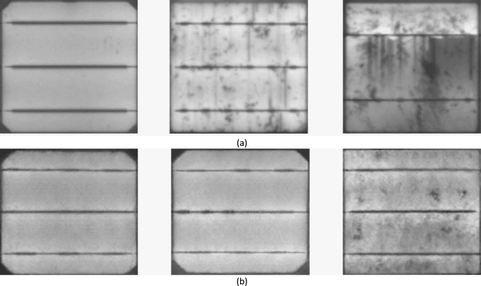
Visual comparison between (a) real and (b) GAN-generated electroluminescence (EL) images.
One-cycle policy
The one-cycle strategy proves highly effective when training complex models, delivering rapid results. It leverages the Cyclical Learning Rate (CLR) to achieve faster training times while providing regularization benefits with minimal modifications. By selecting optimal learning rates at each iteration, the model can converge quickly.
This strategy implements a cycle shorter than the total number of iterations/epochs, allowing the learning rate to decrease by several orders of magnitude below the initial rate during remaining iterations. The CLR philosophy effectively combines curricular learning with simulated annealing approaches. For certain hyper-parameter values, using extremely high learning rates with the CLR approach can dramatically accelerate training—up to ten times faster. This remarkable acceleration phenomenon was termed”Super-Convergence”by Leslie Smith61.
Changing learning rates
According to the research62, a cycle with two equal-length steps is recommended, with the first step increasing from a lower to a higher learning rate and the second step returning to a minimum. It is worth noting that the growth and reduction change in a linear fashion. The maximum learning rate should be determined using the learning rate finder tool. For the minimum learning rate, it can be set to approximately 1/3 or 1/4 of the maximum rate. The lowest learning rate should then be reduced further by a factor of 10 from this minimum value. The cycle length should be configured to be shorter than the total number of training epochs. This structure ensures that the final epochs will operate with a learning rate that’s several orders of magnitude lower than even the lowest specified rate in the cycle, allowing for fine-tuning and convergence at the end of training.
Architecture for deep transfer learning
Deep learning is a ML subfield inspired by brain structure. In recent years, these approaches have shown exceptional performance in PV cell image processing. Applying deep learning algorithms to PV data aims to extract valuable insights. These models have successfully been used across various applications including classification, segmentation, and lesion identification in PV cell data.
PV cell imaging techniques like IR imaging and EL imaging are analyzed using deep learning models to examine image and signal data. These investigations help detect and categorize defects including micro-cracks, finger failure, silicon material defects, cell connectivity deterioration, and electrical separation or recognition problems63.
In convolutional neural network (CNN) processing, the system first encodes input images into numerical matrices for computational processing. This matrix representation enables the network to establish correlations between image transformations and their corresponding labels. Through iterative training, CNN learns to associate specific spatial patterns with classification outcomes, building predictive capabilities for new images.
The fundamental CNN architecture comprises three core components arranged in sequence64:
-
1.
Convolutional Layers: Perform feature extraction through learned filters that detect spatial hierarchies of patterns
-
2.
Pooling Layers: Reduce dimensionality while preserving critical features through operations like max-pooling
-
3.
Fully Connected Layers: Integrate extracted features for final classification decisions
This layered architecture progressively transforms raw pixel data into increasingly abstract representations, enabling effective pattern recognition while maintaining spatial relationships within the input data.
Convolutional layer
The convolutional layer constitutes the fundamental building block of CNN architectures, performing localized feature extraction through learned filter operations. These layers systematically identify and quantify distinctive spatial patterns by computing dot products between small receptive fields and convolutional kernels (filters). The process generates feature maps that encode hierarchical representations of the input data, with early layers capturing basic visual elements (edges, textures) and deeper layers detecting increasingly complex patterns. When an image is provided as input, this layer applies filters to process it. The filtering operation produces values that collectively form a feature map. Within this layer, kernels (small matrices) slide across the pattern to capture both simple and complex information65. These kernels, typically sized as 3 × 3 or 5 × 5 matrices, transform the input pattern through matrix operations. The stride parameter defines how many steps the kernel takes when moving across the input matrix. The result of the convolutional layer may be stated as:
$${X}_{j}^{l}=f(sum_{a=1}^{N}{w}_{j}^{l-1}*{y}_{a}^{l-1}+{b}_{j}^{l})$$
(3)
where ({X}_{j}^{l}) is the ({j}^{th}) feature map in layer l, ({w}_{j}^{l-1}) indicates jth kernels in layer (l-1), ({y}_{a}^{l-1}) represents the ath feature map in layer (l-1), ({b}_{j}^{l}) indicates the bias of the (jth) feature map in layer l, N is the number of total features in layer (l-1), and (∗) represents the vector convolution process64.
Pooling layer
Following the convolutional layer is the pooling layer. This layer’s purpose is to decrease the number of feature maps and network parameters by applying specific mathematical operations. The research66 employs both maximum pooling and global average pooling techniques. The max-pooling operation downsamples feature maps by extracting only the maximum activation value within each n*n sliding window (typically 2*2), producing more compact representations while preserving the most salient features. This spatial reduction (1) decreases computational complexity and (2) provides basic translation invariance. The architecture incorporates two additional critical layers:
-
1.
Global average pooling (GAP):
-
o
Replaces flattening operations before the fully connected layer
-
o
Reduces each feature map to its spatial meaning
-
o
Generates 1D feature vectors while maintaining spatial relationships
-
o
-
2.
Dropout layer:
-
o
Randomly deactivates neurons during training (typically with p = 0.5)
-
o
Creating an implicit ensemble effect
-
o
Effectively regularizes the network by preventing co-adaptation of features
-
o
Fully connected layer
The fully connected layer represents the final and most crucial component of CNN architecture. This layer operates as a multilayer perceptron. Within fully connected layers, the rectified linear unit (Relu) activation function is commonly implemented, while the SoftMax activation function is applied to predicted output images in the final layer of the fully connected section. The mathematical formulations for these two activation functions would follow:
$$text{Relu}left(text{x}right)=left{begin{array}{c}0,quad if x<0\ x, quad if x ge 0end{array}right.$$
(4)
$$text{Softmax}left(text{x}right)=frac{{text{e}}^{{text{x}}_{text{i}}}}{sum_{text{y}=1}^{text{m}}{text{e}}_{text{y}}^{text{x}}}$$
(5)
where ({x}_{i}) and (m) represent the input data and the number of classes, respectively. Within a fully connected layer, each neuron maintains complete connections to all activation functions from the preceding layer.
Pre‑trained models
Training convolutional neural networks (CNNs) with millions of parameters from scratch demands significant computational resources and time. To mitigate these challenges, transfer learning has emerged as an effective strategy, where knowledge (weights and parameters) from models pre-trained on large datasets (e.g., ImageNet) is transferred to new tasks67,68. This approach focuses learning on newly added task-specific layers while preserving the transferred feature extraction capabilities, significantly reducing training time and computational costs—particularly beneficial for limited datasets69. A critical challenge in photovoltaic (PV) cell analysis is dataset scarcity. While deep learning traditionally requires extensive labeled data, manual annotation is costly and labor-intensive. Transfer learning addresses this by leveraging pre-trained models’ learned features, enabling effective training even with smaller datasets.
In this study, we implemented deep CNN-based architectures—including DenseNet169, DenseNet201, ResNet101, ResNet152, SENet154, VGG16, and VGG19—to classify electroluminescence (EL) images of PV cells into defective and non-defective categories. To further compensate for data limitations, we integrated generative adversarial network (GAN)-based augmentation, synthetically expanding the training dataset. Figure 4 illustrates the proposed framework, which combines pre-trained models with augmented data for optimized defect detection. In addition to showing model architecture, Fig. 3 also summarizes the overall system workflow, including input, augmentation, model training, and classification output, providing a clear visual overview of the proposed methodology.
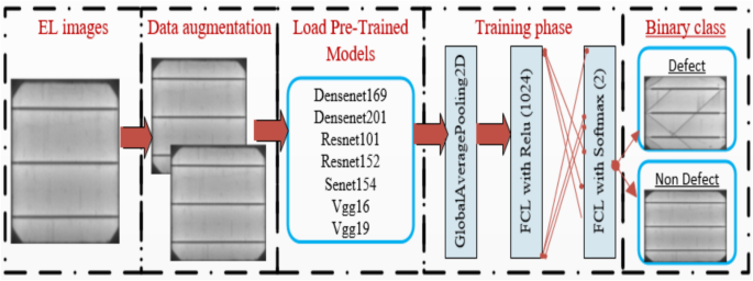
Architecture of pre-trained models for defect and Non-defect EL image prediction, illustrating the overall system workflow.
Densenet-169 and densenet201
DenseNet-169 and DenseNet-201 are part of the DenseNet model family, widely used for image classification tasks. The primary distinction between DenseNet-201 and other models in the series lies in their size and accuracy. DenseNet-201 is marginally larger, with a size of approximately 77MB, compared to DenseNet-169, which is around 55MB. Initially trained using Torch, these models were later converted to the Caffe* framework. All DenseNet variants were pre-trained on the ImageNet image dataset. The models accept input as a blob representing a single image with dimensions 1 × 3 × 224 × 224 in BGR format. Before feeding the image into the network, the mean BGR values [103.94, 116.78, 123.68] should be subtracted, and the resulting values should be scaled by dividing by 0.017. Both DenseNet-169 and DenseNet-201 generate standard classification outputs across 1000 categories, consistent with the ImageNet dataset classifications70,71.
Senet154
SENet-154 is an upgraded version of 64*4d ResNeXt-152 that incorporates SE blocks and distributes the original ResNeXt-101 using ResNet-152’s block stacking approach72,73.
Vgg16 and Vgg19
Vgg16 and Vgg19 are both convolutional neural network architectures with minimal differences between them apart from their layer depth. The VGG-16 model represents a convolutional neural network that underwent training on more than one million images from the ImageNet database. This network contains 16 layers and can classify images across 1000 different object categories, including keyboards, mice, pencils, and various animals. The network requires input images with dimensions of 224 by 224 pixels. Vgg19 follows the same architectural principles as Vgg16, with the primary distinction being its increased depth of 19 layers. Regardless of the specific version, both networks analyze image objects using convolutional neural network methodology68,74.
ResNet101 and ResNet152
The architectures of ResNet101 and ResNet152 contain 101 and 152 layers respectively, achieved through layered ResNet building blocks. A pre-trained version of this network exists in the ImageNet database, having undergone training on more than a million images. This extensive training has enabled the network to develop sophisticated feature representations applicable to diverse image types. The network requires input images sized at 224 × 224 pixels68,75.
Experimental setup
The implementation of the proposed deep transfer learning models was conducted using Python programming language. All experimental testing was performed on a Google Collaboratory (Colab) Linux server running Ubuntu 16.04 operating system, utilizing the free online cloud service with hardware options including Central Processing Unit (CPU), Tesla K80 Graphics Processing Unit (GPU), or Tensor Processing Unit (TPU). For the GAN hyperparameters shown in Table 5, an optimal batch size of 32 was selected for the GAN model, along with 100 epochs and a 0.0002 learning rate. The CNN architectures (Densenet169, Densenet201, Resnet101, Resnet152, Senet154, Vgg16, and Vgg19) underwent pre-training with random initialization weights by optimizing the cross-entropy function using the adaptive moment estimation (ADAM) optimizer (with parameters β₁ = 0.9 and β₂ = 0.999). ReLU activation functions were implemented throughout all convolutional layers.
In one approach, we used a batch size of 16 with a learning rate of 0.004, while in the alternative approach, the learning rate was determined by the“find_lr”function from the fastai Python library. For all experiments, the number of epochs was empirically set at 70. The datasets were randomly split into two segments: 80% allocated for training and 20% reserved for testing.
Performance evaluation metrics
To assess the algorithms’ performance, the following measures are used:
where ({t}_{p}) is the number of true positives and ({f}_{n}) the number of false negatives.
At β = 1, the F1-score is evenly balanced. It prioritizes accuracy when β > 1 and recall otherwise. The F1-score may be seen as a weighted average of accuracy and recall45,64.