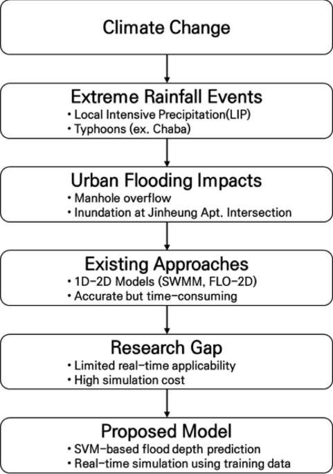
Estimation of precipitation under given return periods. The frequency-based precipitation values used in this study were derived from the Seoul (108) meteorological station. Rainfall frequency analysis was performed using maximum observed rainfall depths for durations ranging from 10 minutes to 24 hours. The analysis was conducted using the Frequency Analysis for Rainfall Data software(FARD 2006), developed by the National Disaster Management Research Institute (NDMI) of Korea. The software is freely available at the official NDMI website: https://www.ndmi.go.kr (in Korean). FARD 2006 supports the application of 13 different probability distributions (e.g., Gumbel, GEV, Lognormal) and performs statistical goodness-of-fit tests29. Based on evaluation criteria including the chi-squared (χ2) test, Kolmogorov–Smirnov test, Cramer–von Mises test, and PPCC, the Gumbel distribution was selected as the most suitable model. This approach follows the methodology presented in the national guideline “Improvement and Supplementation of Probable Rainfall Maps” by the Ministry of Land, Transport and Maritime Affairs30.
It is a fact that there is no measurement data available to directly predict flood depth based on actual rainfall. Therefore, to predict flood depth using the SVM model, the probability of precipitation according to the return period was estimated as shown in Table 2.
The temporal rainfall distribution was determined using the 3rd quartile of the Huff method, which divides a storm event into four quartiles based on the timing of peak rainfall. The method expresses cumulative rainfall and time in dimensionless ratios, allowing generalization across storm durations. The 3rd quartile reflects mid-duration peak rainfall, which is representative of typical urban storm events.
To construct the dimensionless cumulative rainfall curve, two ratios are defined. The dimensionless cumulative time at an arbitrary time step (T(i)) is given as:
$$PT(i)=frac{T(i)}{text{TO}}times 100%$$
(16)
where (T(i)) denotes the elapsed time from the beginning of the rainfall to the (i)-th interval, and (TO) is the total rainfall duration.
Likewise, the dimensionless cumulative rainfall is calculated as:
$$PR(i)=frac{R(i)}{text{RO}}times 100%$$
(17)
where (R(i)) is the cumulative rainfall up to time (T(i)), and (T(O)) is the total rainfall over the entire storm event. These non-dimensional expressions enable the application of the Huff method to diverse design scenarios and support the generation of realistic synthetic hyetographs.
The estimated precipitation was used as input data and applied to SWMM, a runoff analysis model. As a result, overflow occurred in 22 manholes at the 30-year return period, 25 manholes at the 50-year return period, and 31 manholes at the 100-year return period. Finally, based on the results of the runoff analysis, the critical manhole points that most affect the flood depth are shown in Table 3.
After applying the results of the runoff analysis as the boundary condition of the 2D flood model, the flood analysis was performed. As a result, it was confirmed that flooding occurred around Gangnam Station and the intersection of Jinheung Apartment, which is a regularly flooded area, as seen in the previous flooding patterns based on actual rainfall in Fig. 10.
Flood for probabilistic precipitation, map generated in the ArcGIS 10.1 (ESRI, https://www.esri.com/).
SVM model application. In this study, the prediction model of the SVM model was used. The parameters were calculated through pattern search, and flood depth was predicted based on precipitation and manhole overflow using the training process and verification.
As a result of the 2D inundation analysis, the intersection of Jinheung Apartment in Gangnam, where the inundation depth was the largest, was selected as the target basin. The results of the 2D inundation analysis with a return period of 100 years were used to predict the depth of flooding. To establish the basic data for the SVM model, rainfall durations ranging from 1 to 5 hours, corresponding to the 100-year return period of precipitation, were selected. Additionally, the amount of manhole overflow based on rainfall time was converted into data through runoff analysis. Subsequently, flood depth data at the intersection of the Jinheung Apartment were calculated through 2D flood analysis, and the results were converted into usable data. Compared to the 2D hydraulic model, which required approximately 3 hours to complete a single simulation including pre-processing and post-processing, the trained SVM model was able to predict flood depth at the target location within a few seconds. This significant reduction in computation time demonstrates the practical efficiency of the proposed framework for near real-time flood forecasting in urban areas. Finally, the estimated data were applied to the SVM model, and the training and verification process was repeated, enabling prediction of flood depth at intersection of the Jinheung Apartment over time.
In this study, the term “real-time prediction” refers to the rapid simulation process of a pre-trained SVM model, which generates flood depth predictions within seconds. Unlike online learning models that require continuous updating and may introduce latency, the pre-trained architecture is intentionally designed for fast and stable deployment in real-time forecasting systems. This approach ensures consistent performance and minimal computation time when responding to imminent rainfall events in urban flood-prone areas.
Since detailed observed flood depth time-series data were not available for the study area, the 1D–2D hydraulic model (SWMM–FLO-2D) was not used as a real-time prediction tool, but instead to generate physically consistent datasets for training the machine learning model.
The training input and verification input data were configured to predict the flood depth. The input variables of the SVM model are cumulative rainfall and cumulative overflow, while the output variable is flood depth. The training dataset was generated from 1-hour to 5-hour rainfall scenarios based on the Huff 100-year return period distribution, recorded at 1-minute intervals. As a result, 190 time-step samples were used for training, and an additional 48 time-step samples were used for model validation. Each time-step sample is structured as a one-dimensional vector, where the cumulative rainfall and overflow serve as input features and the corresponding flood depth serves as the target output.
Firstly, the training data, which includes cumulative precipitation, shows the precipitation duration ranging from 1 to 5 hours according to the 100-year return period in Fig. 11. The amount of overflow at each hour for the manhole at point 3, which significantly influences the intersection of Jinheung Apartment, was calculated through the runoff analysis, and presented in Fig. 12. Finally, through the 2D inundation analysis, the time-dependent inundation depth at the intersection of Jinheung Apartment was computed in Fig. 13. In other words, as can be seen in Figs. 11, 12 and 13, the training data used are hourly rainfall, manhole overflow, and flood depth data for 1 hour, 2 hours, 4 hours, and 5 hours.
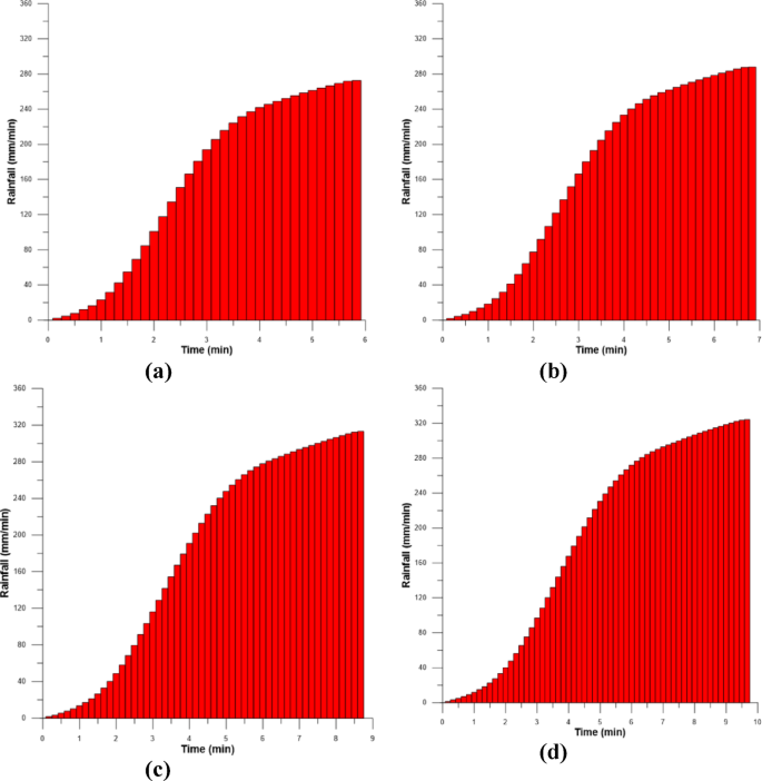
Cumulative precipitation (Huff 100year): a 1hr; b 2hr; c 4hr; d 5hr.
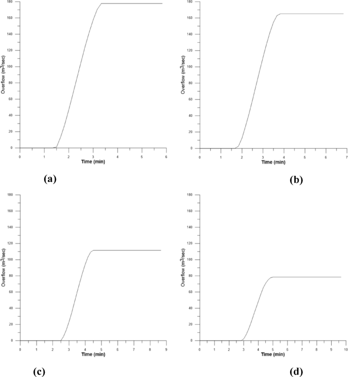
Cumulative overflow at manhole (Huff 100year): a 1hr; b 2hr; c 4hr; d 5hr.
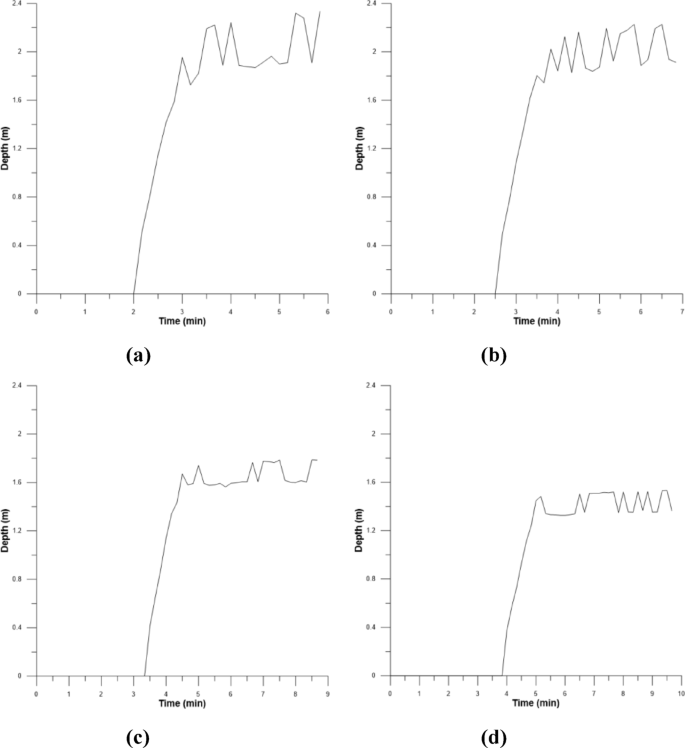
Flood depth at Jinheung Apartment Intersection (Huff 100year): a 1hr; b 2hr; c 4hr; d 5hr.
Second, for the verification data, the cumulative precipitation for a 3 h rainfall duration according to the 100-year return period was selected. Additionally, the overflow and flood depth of the manhole at point 3, which significantly influences the intersection of Jinheung Apartment, were also selected in Fig. 14.
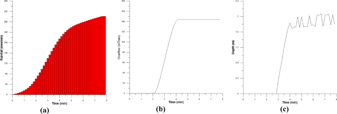
Verification data (Huff 100year, 3hr): a Cumulative precipitation (3hr); b Cumulative overtopping at manhole; c Flood depth at Jinheung Apartment Intersection
Finally, in the SVM model, the cumulative precipitation and cumulative overflow for each hour of precipitation duration from 1 to 5 hours were applied as training data, and the flood depth was repeatedly learned in Fig. 15. Subsequently, the cumulative rainfall and cumulative overflow for each hour of the 3 h rainfall duration in the target basin were input as predicted data, and the flood depth in the target basin was predicted and verified over time in Fig. 16. In Figs. 15 and 16, the X-axis represents time, and the Y-axis represents flood.
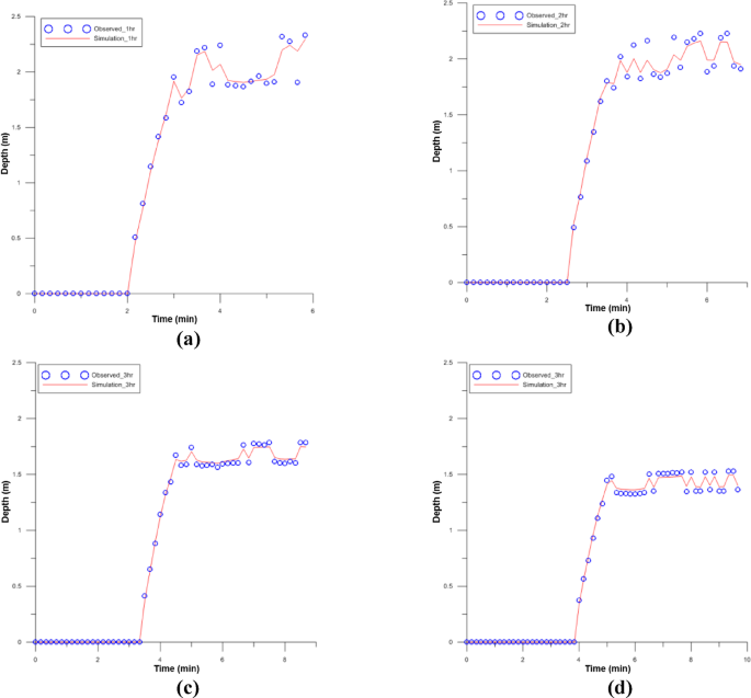
Training results (Huff 100year): a 1hr; b 2hr; c 4hr; d 5hr.
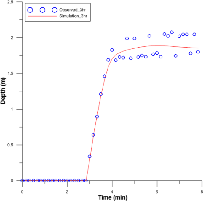
Prediction flood depth (Huff 100year, 3hr).
The results of applying the SVM model showed a similar pattern to the results of the 2D inundation analysis in Fig. 15. Additionally, the predictions of flood depth over time in the target watershed were also similar.
In the results of flood depth prediction over time in Fig. 16, some fluctuations in the measured values occurred at the end. These fluctuations were attributed to the influence of topography, such as buildings and roads. To verify the SVM prediction results from Fig. 17. The average flood depth of the observed values for that segment was 1.87 m, and the average flood depth of the predicted result was 1.86 m, confirming a slight error of 1 cm. Fig. 17a presents the results before calibration, while (b) shows the results after calibration.
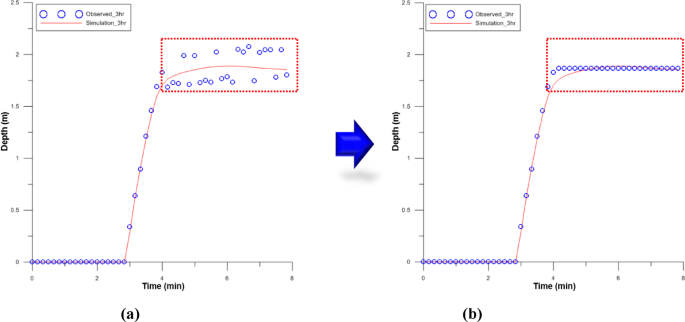
Verification result before and after calibration (Huff 100year_3hr).
Review of the suitability of the SVM model. To assess the suitability of the SVM prediction model, Coefficient of Determination (R2), Nash and Sutcliffe Efficiency (NSE), % Difference, and Root Mean Square Error (RMSE) analyses were performed. The coefficient of determination ranges from 0.0 to 1.0, with higher values indicating a stronger correlation between the measured and simulated values. NSE value approaches 1 when the simulated value is a perfect fit and approaches 0 when the simulated value is merely the average of the measured values. % difference is a statistical value used to compare actual and simulated values mathematically and indicates the reliability of repeated measurements where identical results are expected in Table 4.
$$text{NSE} = 1 -frac{sum_{text{i} = 1}^{text{n}}({text{O}}_{text{i}}-{text{P}}_{text{i}}{)}^{2}}{sum_{text{i} = 1}^{text{n}}({text{O}}_{text{i}}-{text{O}}_{text{Ai}}{)}^{2}}$$
(19)
$$text{%} text{difference} = frac{|sum_{text{i} = 0}^{text{n}}{text{O}}_{text{i}}-sum_{text{i} = 0}^{text{n}}{text{P}}_{text{i}}|}{sum_{text{i} = 0}^{text{n}}{text{O}}_{text{i}}}times 100$$
(20)
$$text{RMSE}= (sum_{text{i} = 1}^{text{n}}frac{{text{P}}_{text{i}}-{text{O}}_{text{i}}}{text{n}}{)}^{1/2}times 100$$
(21)
where, ({P}_{i}): Simulated value; ({O}_{i}): Measured value; (n): Number of data; ({O}_{Ai}): Average of Measured value
As a result of error analysis on the training results, the coefficient of determination was 0.997, the NSE was 0.997, and the % Difference was 0.195, indicating that the confidence interval and acceptable range were very good. The RMSE was 0.044, suggesting the model accurately reflected the measured and simulated values in Table 5.
Regarding the verification results, the coefficient of determination was 0.988, the NSE was 0.987, and the % Difference was 1.080, indicating that the confidence interval and acceptable range were still very good. The RMSE was 0.098, validating the appropriateness of the actual measured values and predicted results of the SVM model in Table 6.
