We first show how breakage–replication/fusion converts free DNA ends into breakpoints on rearranged sequences and then show how breakage–replication/fusion of chromosome fragments produces segmental copy-number gains and amplifications. We place particular emphasis on distinguishing the genomic feature of a rearranged DNA sequence (for example, breakpoints) from the molecular feature of the ancestral chromosome (for example, DNA ends). See Supplementary Note, Section 1 for the complete list of definitions.
Rearrangements from breakage–replication/fusion of DNA ends
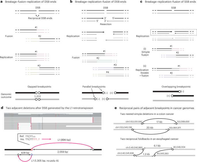
A DNA double-strand break (DSB) generates two reciprocal DNA ends (Fig. 1a). In the G1 phase, these ends can undergo classical non-homologous end-joining (c-NHEJ): they can be ligated together, creating a rearranged sequence with small deletions (or less frequently, duplications), or ligated to DNA ends from distal sites, creating translocations29,30. In either scenario, the ancestral DNA ends are converted to two breakpoints (open circles in Fig. 1a) separated by a small gap, which we term adjacent gapped breakpoints. As the ligation(s) occur before replication, the rearranged DNA sequences are preserved in both sister chromatids after replication. This cascade of events defines the breakage–fusion–replication sequence (Supplementary Video 2).
In a–c, the two strands of the ancestral DNA are shown in black and gray: thick lines represent template DNA strands, thin lines represent newly synthesized DNA strands and arrows represent 3′ ends. Light-colored lines represent distal DNA sequences that are ligated to DSB ends derived from the original DNA. In the genomic outcomes, rearranged DNA is colored (black or gray) according to the ancestral DNA strand, and (−) and (+) denote the orientation of breakpoints defined by the directionality of copy-number transitions from left to right. Examples shown in d and e demonstrate the breakage–replication–fusion mechanism as shown in b. a, Breakage–fusion–replication of DSB ends. A single DSB generates two reciprocal DSB ends; each end is fused to a distal DNA end before replication (#1, #2), creating two reciprocal breakpoints separated by a small gap (open circles), termed adjacent gapped breakpoints. Note that after replication, both sister chromatids (black and gray) have the same breakpoints. b, Breakage–replication–fusion of DSB ends. Two DSB ends created by a single DSB undergo resection and replication, creating two pairs of replicated (sister) DNA ends that may undergo further end processing (not shown). Fusions of these DNA ends to distal DNA ends create four breakpoints in the rearranged sequences, one from each ancestral ssDNA end (5′ or 3′). Breakpoints derived from the 5′ end and 3′ end of a single ancestral DSB end (for example, #1 and #2) are adjacent and have the same orientation, termed adjacent parallel breakpoints. c, Breakage–replication–fusion of single-strand break (SSB) ends. Two ssDNA ends on the black strand are converted to two DSB ends by replication (dashed box). (i), The two DSB ends undergo simple fusions to create two gapped breakpoints, as in a. (ii), The DSB ends initiate homologous recombination using the intact sister chromatid (gray), creating two breakpoints with a small overlap by over-replication (replication bypass); we refer to these as adjacent overlapping breakpoints. The example here also shows a sister-chromatid exchange (breakpoint #2 is now on the gray chromatid). See Extended Data Fig. 8c for additional information. d, Two adjacent deletions resulting from a single DSB owing to L1 retrotransposition in an experimentally generated clone of RPE-1 cells. These are the only L1 insertions identified on this chromosome (chr14) in this clone. The deletions are supported by long reads (top) and define two pairs of adjacent breakpoints (bottom). Each deletion junction contains a truncated L1 insertion and joins two DNA ends derived from a single ancestral strand (black or gray); the polarity of each ancestral strand is determined from the directionality of the reverse-transcribed L1 (complementary to the L1 messenger RNA, magenta arrows). The red circle (chr14:50,762,606) marks the ancestral 3′ end that underwent target-primed reverse transcription: this is established by the poly-T sequence (in red in the insertion sequence junction (Ins.)) that marks the initiation of reverse transcription and by the ORF2p EN target sequence at the breakpoint (TTcTT|aa in the reference sequence (Ref.)). The blue circle below the red (chr14:50,762,603) is derived from the 3′ end on the opposite strand that also underwent reverse transcription initiated from an internal position of the L1 mRNA, showing no poly-A/T. The two distal breakpoints (black circles) are inferred to be derived from the resected 5′ ends. e, Two examples of reciprocal breakpoint pairs in cancer genomes identified from the rearrangement junctions from a previous publication16. Top: two nested simple deletions in a colon cancer that are similar to d but without insertions. Bottom: two reciprocal foldbacks (direct joining of parallel breakpoints from each side) in an esophageal cancer. Note that the ancestral strand of each rearranged DNA segment cannot be definitively determined solely based on the breakpoints, as some DSB ends may have 5′ overhangs. Therefore, the rearranged DNA segments are all shown in gray.
If the DSB ends have substantial overhangs that prevent c-NHEJ31,32 (for example, because of 5′-resection33,34,35 or 3′-exonuclease degradation24), they can remain unligated during G1 and persist into S phase. During S phase, these ends, like broken chromosome ends36, are replicated to generate two ‘sister’ DNA ends. Ligations of these replicated DNA ends can generate up to four rearrangement junctions (Fig. 1b). This cascade of events defines the breakage–replication–fusion sequence (Supplementary Video 3). In breakage–replication–fusion, a staggered DNA end is converted into two adjacent but non-identical breakpoints with the same orientation, which we term adjacent parallel breakpoints. When the sister DNA ends are directly ligated to each other, it produces a ‘foldback’ junction, joining two adjacent parallel breakpoints. Foldback junctions are often assumed to indicate fusions between the ends of broken sister chromatids in BFB cycles37,38; later, we will show that such fusions also occur between sister DNA fragments.
In a variation of breakage–replication–fusion, two single-strand DNA (ssDNA) ends with a small gap are converted into two reciprocal DSB ends by replication39,40 (Fig. 1c). These two DSB ends can generate two rearrangement breakpoints with either a small gap (i) or a small overlap (ii) by a replication bypass mechanism18,41,42. We refer to the latter as adjacent overlapping breakpoints.
A single DSB end undergoes either breakage–fusion–replication or breakage–replication–fusion. However, when a catastrophic event creates many DNA breaks, some will undergo breakage–replication–fusion while others will undergo breakage–fusion–replication; we refer to the latter as the breakage–replication/fusion cycle.
Adjacent parallel breakpoints from DNA end replication
We first sought experimental evidence that a single DNA end can generate two adjacent parallel breakpoints. We exploited L1 retrotransposition to simultaneously generate and mark DSB ends. As described in a separate paper43, transient L1 expression in p53-null RPE-1 cells generated both L1 insertions and translocation junctions containing reverse-transcribed L1 sequences. Both outcomes originate from DSB ends generated by the L1 open reading frame 2 protein (ORF2p), and are identified by the insertion of reverse-transcribed sequences (the ‘primary’ end of retrotransposition) and/or the presence of ORF2p endonuclease target sequences near the break site.
We identified multiple instances of adjacent parallel breakpoints in clones generated after L1 induction that had features indicating an origin from ORF2p-induced DSBs (Supplementary Note, Section 6). In the example shown in Fig. 1d, two nested deletions, each containing a truncated L1 insertion, indicate two pairs of adjacent parallel breakpoints (Fig. 1b). The sequence features at the two closest breakpoints (red and blue circles) directly relate them to L1 ORF2p, and the distances between each pair of parallel breakpoints (429 bp and 2,059 bp) are consistent with DSB resection33,34,35. Together, these observations demonstrate that breakage–replication–fusion can generate two parallel breakpoints from a single DSB end.
Footprints of DNA end replication in human disease genomes
We next sought evidence of DSB end replication in human disease genomes. Although we cannot directly relate a rearrangement breakpoint to an ancestral DNA end, we can identify an ancestral DSB from breakpoints derived from reciprocal DSB ends: in particular, a reciprocal pair of parallel breakpoints directly identifies reciprocal DSB ends that undergo breakage–replication–fusion (Fig. 1b,d).
Based on the observations from the L1 clones (Fig. 1d and Supplementary Note, Section 6), we selected a heuristic threshold distance of 20 kb for the identification of adjacent parallel breakpoints (Methods). From 592,176 breakpoints detected in 2,588 cancers by the Pan-Cancer Analyses of Whole Genomes (PCAWG) study16, we identified 20,795 pairs of adjacent parallel breakpoints from 1,793 samples. These breakpoints were identified at 35,422 rearrangement junctions (12% of all junctions), including 7,393 foldback junctions. Thus, adjacent parallel breakpoints are a widespread feature in cancer genomes.
For 3,138 pairs of adjacent parallel breakpoints, we identified one or multiple reciprocal breakpoints that demonstrate their origin from ancestral DSBs. There were 417 instances of reciprocal parallel breakpoints as shown in Fig. 1b. Among these were 53 instances of nested deletions (Supplementary Table 1) and 23 instances of reciprocal foldbacks (Supplementary Table 2), with examples shown in Fig. 1e. In the remaining instances, one or multiple breakpoints formed long-range translocations. Examples of reciprocal foldbacks were previously noted in ovarian cancers (supplementary fig. 8f of a previous publication44) but were assumed to result from BFB cycles. We suggest that these events arise from reciprocal DSB ends undergoing breakage–replication–fusion.
We further assessed the probability that adjacent parallel breakpoints were generated independently based on the distance between these breakpoints and their distance to the nearest breakpoint on the opposite side (Methods). This analysis showed that for 16,132 of 20,795 pairs of adjacent parallel breakpoints, the probability that they were generated independently was less than 5%.
In summary, adjacent parallel breakpoints are common in cancer genomes, and our analysis suggests that many of them are derived from sister DNA ends generated by breakage–replication–fusion.
DNA duplication and amplification from breakage–replication/fusion
When the sister DNA ends are joined together in a single rearranged chromosome, this rearranged chromosome will contain a duplication (Fig. 2a). Moreover, the duplicated segments will be bounded by adjacent parallel breakpoints derived from sister DNA ends. Consistent with this prediction, we identified examples of copy-number gains flanked by adjacent parallel breakpoints in both human cancers and congenital diseases14,15,45,46 (Extended Data Fig. 1 and Supplementary Note, Section 7).
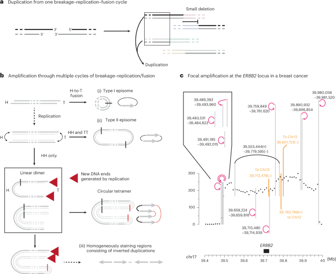
a, A single breakage–replication–fusion cycle can lead to DNA duplications when two sister DNA fragments are retained in a single rearranged chromosome and segregated into one cell. See Extended Data Fig. 1 for examples from human disease genomes. b, Three processes of amplification from an acentric DNA fragment. (i), A head (H)-to-tail (T) junction (black vertical line) joining opposite ends of the DNA fragment creates a type I episome. (ii), Fusions between sister DNA ends on opposite sides of replicated DNA create a type II episome. In both scenarios, the ‘episome’ (acentric extra-chromosomal circles) can be amplified by uneven segregation. (iii), If sister-end fusion occurs on one side (head-to-head, black vertical line) of replicated DNA, and sister ends on the opposite side remain unligated (red arrows), the outcome is a double-sized linear DNA fragment. Iterations of the same process can create a large array of amplified DNA with only head-to-head and tail-to-tail junctions (later fusion junctions shown as red vertical lines). The amplified DNA can be either circular or linear and consists of only inverted duplications. In the schematic diagrams of amplified DNA on the right, the original DNA sequence is shown as a gray arrow to highlight the relative orientation of duplicated DNA. c, Amplification of the ERBB2 oncogene in the HCC1954 genome that is consistent with linear DNA amplification as shown in b. The copy-number plot shows total sequence coverage in 10 kb bins. Breakpoints forming long-range rearrangement junctions are shown as vertical lines (three breakpoints joining chr12 are shown in orange); curved arrows represent foldback junctions between adjacent parallel breakpoints (positions labeled next to the curved arrows). See Supplementary Note, Section 7 for the copy-number data and rearrangement junctions of the entire chr17. Consider the three foldback junctions near 39.5 Mb within the 0.5 Mb amplicon: if they were generated by BFB cycles, the location of each foldback junction would correspond to the break site of a different dicentric chromosome bridge; the probability of generating two additional breaks within 10 kb from the first break is (10 kb / 0.5 Mb)2 = 0.0004. Also note the proximity between the breakpoint at chr17:39,713,478 and the foldback junction between chr17:39,713,480 and 39,714,939.
Foldback junctions are the simplest outcome when sister DNA ends are joined together. We envision two processes by which a double-stranded DNA (dsDNA) fragment can generate amplification with only foldback junctions (Fig. 2b). If both ends of a dsDNA fragment undergo breakage–replication–fusion to form foldback junctions (Fig. 2b (ii)), the outcome is a dimeric circular DNA (previously termed type II episomes47). Like simple monomeric DNA circles (type I episomes47; Fig. 2b (i)), dimeric DNA circles can fuel DNA amplification by asymmetric segregation over successive generations. This model explains the amplification at the AR locus flanked by foldback junctions in a castration-resistant prostate cancer46 (Extended Data Fig. 1a, right). Amplification can also occur on a linear acentric DNA fragment when the DNA ends on opposite sides fuse asynchronously (Fig. 2b (iii)). If sister DNA ends on one side are fused together, but sister DNA ends on the opposite side remain unligated (red arrows), the product is a linear inverted dimer. In the next cell cycle, another round of replication–fusion can create a circular or linear tetramer without any new breakage. Iterations of this process will produce a large tandem array of amplified DNA with ‘nested’ foldbacks that form homogeneously staining regions of inverted duplications48,49.
One such example is the amplification spanning the ERBB2 oncogene in the HCC1954 breast cancer genome (Fig. 2c). Similar patterns were also found in chr8p, chr12p and chr20q in this genome (Extended Data Fig. 2a–c and Supplementary Tables 3 and 4). Here, amplified ERBB2 is contained in homogeneously staining regions37,50 and is bounded by multiple foldback junctions previously attributed to BFB cycles37. However, the probability of generating foldback junctions in such close proximity by successive BFB cycles is very small (see Fig. 2c caption). Under the breakage–replication/fusion model, the close proximity between foldback junctions near 39.5 Mb is a natural consequence of the close proximity between the 3′ and 5′ ends of an ancestral DSB end (Fig. 2b (iii)). Moreover, if amplification takes place on a linear, extra-chromosomal DNA fragment, secondary breakpoints (both foldbacks and long-range breakpoints) can only arise within the amplicon, thus explaining the concentration of breakpoints within the amplified region (39.5–40 Mb). Importantly, in linear DNA amplification, amplified DNA is automatically doubled and linked in one chromosome that is segregated into one daughter cell, thus providing a more rapid route to higher DNA copy number than amplification by random segregation of episomal circles. The amplification of DNA copy number also does not require selection during the intermediate steps of amplification; therefore, focal amplifications lacking oncogenes (Extended Data Fig. 2a–c) may be passengers that undergo clonal fixation.
In summary, the presence of duplicated or amplified DNA segments flanked by adjacent parallel breakpoints suggests an origin from breakage–replication/fusion. From a single acentric DNA fragment, breakage–replication/fusion can generate dimeric DNA circles or a linear array of inverted duplications with closely spaced foldbacks, explaining the long-standing observation of inverted duplications in amplified DNA47,48,49 that are unlikely to arise by multi-generational BFB cycles37,38,44.
Segmental copy-number gains after chromosome fragmentation
Above, we described the rearrangement and copy-number outcomes of breakage–replication/fusion occurring at a single dsDNA end and a single dsDNA fragment with two ends. Below, we describe the copy-number and rearrangement outcomes of breakage–replication/fusion after chromosome fragmentation.
We focused the analysis on an experimental model of chromothripsis (Fig. 3a, left) because this system enabled us to determine the structure of rearranged chromosomes with near-complete resolution (Methods). In a previous study21, we used CRISPR–Cas9 to generate chromosome bridges containing dicentric chr4 and derived single cells with a broken chr4 (Supplementary Note, Section 8). In one generation, bridge breakage produced daughter cells with reciprocal DNA retention and deletion21 similar to what was observed immediately after micronucleation20. However, over many generations, clones derived from single cells frequently had subclonal copy-number gains without reciprocal loss in the sibling clone21. The presence of copy-number gains in clones expanded after chromosome fragmentation was also observed in clones expanded after telomere crisis24 (Supplementary Note, Section 9) or micronucleation25 (Extended Data Fig. 3 and Supplementary Table 5).
One bridge clone (primary clone 1a from a previous publication21, hereafter referred to as clone a) is interesting because the bulk DNA copy number oscillates between variable non-integer states that indicate subclonal copy-number variation (Fig. 3a, middle). Moreover, some subclones showed two-state copy number oscillation while others showed segmental copy-number gains (Fig. 3a, right, and Fig. 3b; also see fig. S22 from previous work21). The presence of subclonal copy-number variation enabled us to first determine the breakpoints of duplicated segments and then infer the evolutionary history of the rearrangements that produced the duplications (Methods and Supplementary Note, Sections 10 and 11). Based on a joint analysis of segmental DNA copy number (Supplementary Table 8) and rearrangement junctions (Supplementary Table 9), we determined both the structure (Extended Data Fig. 4) and the joining pattern (Extended Data Fig. 5) of nearly all duplicated segments in the subclones of clone a. In total, we identified 86 rearranged segments with sizes above 10 kb (Supplementary Tables 10–12) and 126 short insertions (<10 kb) between these segments (Supplementary Tables 13–16). We next show that the genomic features of the large segments, the short insertions and their arrangement in the rearranged chromosomes indicate that they all originate from breakage–replication/fusion of a single chromatid.
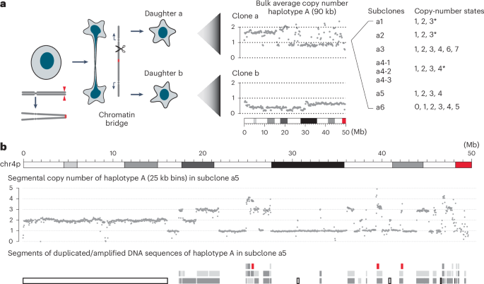
a, Left: experimental workflow; middle: bulk average DNA copy number of the 4A homolog (90 kb bins) in two clones, each derived from a daughter cell after breakage of a dicentric chr4 bridge. Note the non-integer copy-number states that indicate subclonal copy-number heterogeneity in both clones. Right: copy-number states in eight representative single-cell subclones derived from the top clone (clone a). Subclones a1 and a2 show mostly two-state copy-number oscillation (only one segment at three copies, indicated by ∗); a4 shows mostly three-state copy-number oscillation (only one segment at four copies, indicated by *); a5 shows four-state copy-number oscillation; a3 and a6 contain additional amplifications inferred to have been generated by secondary events. See Supplementary Table 8 for the complete segmental copy-number data of all the subclones. b, The copy number (25 kb bins, 4A haplotype) and rearranged segments of chr4p in subclone a5. There is an intact 4p copy in addition to the rearranged segments. Single-copy segments are shown as open bars, duplicated segments inferred to have been derived from sister DNA fragments by breakage–replication/fusion are shown as dark and light gray bars, and triplicated segments are shown as red bars. See Extended Data Fig. 5 for the order of rearranged segments in the rearranged chromosome.
Large duplications from breakage–replication/fusion
The origin of large duplications in clone a from ancestral chromosome fragments that underwent breakage–replication/fusion is established by two orthogonal lines of evidence that relate the boundaries of the duplications to ancestral DNA ends.
First, we identified 18 pairs of duplicated segments that are flanked by identical (‘flush’) or adjacent parallel (‘staggered’) breakpoints within 20 kb (Fig. 4). Knowing the exact size of each duplicated segment, we could assess the probability that the staggered breakpoints were generated independently using the ratio of breakpoint distance to the segmental size (Extended Data Fig. 6). Based on this metric, we determined that for 15 out of 20 pairs of staggered breakpoints, the probability of independent breakpoint generation was less than 0.05 (Supplementary Table 11). For the remaining five pairs, the breakpoint distances were within a similar range but the segments were shorter; therefore, all staggered breakpoints are consistent with an origin from the replication of (hyper)resected DSB ends. For three pairs of segments (Bb1/Bb2, Cb1/Cb2, Cc1/Cc2), the presence of reciprocal breakpoints directly established their origin from chromosome fragmentation (Extended Data Fig. 7a). These data provide statistical evidence that the staggered boundaries of duplicated segments arose from breakage–replication–fusion.
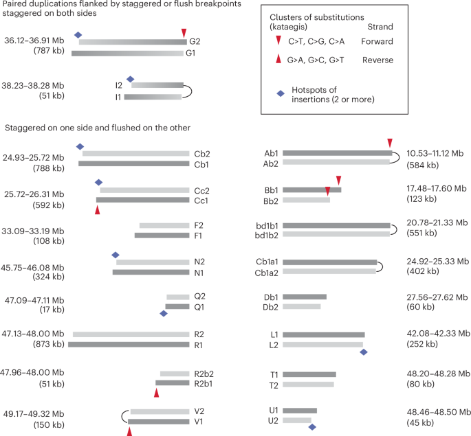
Each bar represents a rearranged segment (also see Extended Data Fig. 4); the coordinates of segmental breakpoints are listed in Supplementary Table 10. Arcs connecting adjacent breakpoints represent foldback junctions. Segmental sizes are labeled, but segments are not shown true to scale. Top: two pairs of duplications with staggered breakpoints on both sides. Dark and lighter ends correspond to boundaries inferred to be derived from ancestral 3′-ssDNA and 5′-ssDNA ends. Bottom: 16 pairs of duplications with flush breakpoints on one side and staggered breakpoints on the other side. Fusions between these segments create compound sister segments as shown in Extended Data Fig. 7c. Segments in darker gray are inferred to be derived from the ancestral DNA strands with a 3′ overhang. Red arrows point to regions with clustered substitutions (kataegis) indicating strand-specific cytosine deamination: downward arrows indicate deamination of cytosines on forward strand DNA (TpC>TpT, TpG or TpA); upward arrows indicate deamination of cytosines on reverse strand DNA (GpA>ApA and so on). Except for the kataegis cluster on the right end of segment Bb2 (explained in Extended Data Fig. 7b), all the other clusters are restricted to the offset region inferred to be the 3′ overhang of the ancestral DNA (dark gray) and show deamination signatures consistent with the DNA strands predicted by the breakpoints. Diamonds indicate regions corresponding to origins of multiple insertions (see Fig. 5).
Second, we observed strand-coordinated base substitutions near the staggered breakpoints that directly established their origin from staggered DSB ends. Based on the breakage–replication/fusion model, the shorter breakpoint derives from an ancestral 5′ end and the longer breakpoint derives from an ancestral 3′ end. Thus, the offset region between the two breakpoints originates from the ancestral ssDNA overhang. We identified seven clusters of substitutions near the staggered breakpoints (Fig. 4, downward or upward arrows), six of which were restricted to the offset region (the only exception near the right side of the shorter Bb2 segment is explained in Extended Data Fig. 7b.) All the substitutions reflect deamination in the TpC context that is consistent with the outcome of ssDNA deamination by APOBEC enzymes51. Importantly, the signature of substitutions (C > X on the right side of each segment, downward arrows; G > X on the left side of each segment, upward arrows) directly established the deaminated ssDNA to be a 3′ overhang. Thus, the pattern of deamination between staggered breakpoints provides molecular evidence for their origin from staggered DSB ends. Additional evidence linking staggered breakpoints to staggered DSB ends comes from the coordination between breakpoints on opposite sides of duplicated segments (Extended Data Fig. 7c and caption).
Based on adjacent parallel breakpoints, we determined that 40 duplicated segments in clone a were derived from ancestral sister DNA fragments generated by breakage–replication/fusion (Supplementary Table 10).
DNA over-replication from breakage–replication/fusion
In addition to nearly identical duplications generated by normal, semi-conservative replication of ancestral chromosome fragments, we also identified rare examples reflecting two mechanisms of DNA over-replication. The replication bypass mechanism41,42 (Fig. 1c) explains two instances of overlapping duplications18,52 (Extended Data Fig. 8a–c and caption); the second mechanism, leading to re-replication of a previously replicated DNA fragment, occurs when the previously replicated segment is fused to an unreplicated segment with unfired origins (Extended Data Fig. 8d and caption).
Short insertions from breakage–replication/fusion
We identified 126 short insertions (median size, 184 bp) at the junctions between large duplications in clone a (Supplementary Tables 13–16). Three pieces of evidence indicate that both the insertions and the insertion rearrangement junctions are generated by chromosome breakage–replication/fusion.
First, when mapped to their origin sites, the insertions displayed several features indicating DNA fragmentation. Nearly all insertions (113 out of 126) were mapped to sites in close proximity (<10 kb) to breakpoints inferred to have been derived from ancestral DNA ends. Moreover, at several sites, the insertions lined up one after another in a tiling pattern, with little gap or overlap (Fig. 5a,b). The tiling pattern of insertions at the origin sites is incompatible with random polymerase template-switching events in MMBIR that are expected to generate duplicated sequences with either large gaps or large overlaps at their original sites (Supplementary Video 4). Finally, seven tiles of insertions were mapped right next to breakpoints derived from the 5′ ends of ancestral DSBs (Figs. 4 and 5b and Supplementary Table 13). Similar patterns were also observed in other experimentally generated clones with chromothripsis (Supplementary Note, Sections 6, 9 and 14), in cancer genomes (Extended Data Fig. 9 and Supplementary Note, Section 7) and in congenital disorders53. Based on these observations, we suggest that many insertions originate as ssDNA fragments complementary to the 3′ overhang of resected DSBs. Two potential models for the generation of these insertions are discussed in Supplementary Note, Section 3.
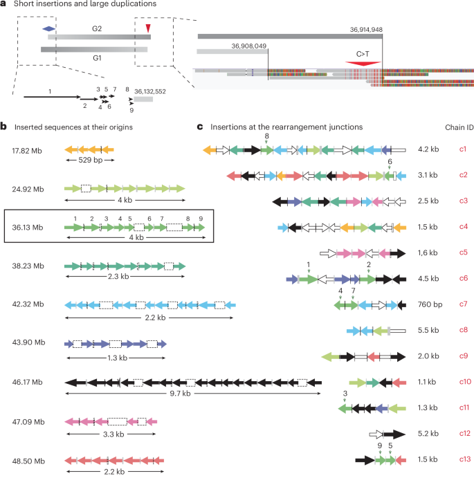
a, An example of nine short insertions mapped to a region adjacent to the left breakpoint of the G2 segment shown in Fig. 4. The sizes and locations of the insertions (black arrows) are shown true to scale. We infer these insertions to have originated as ssDNA fragments of forward strand DNA based on the signature of deamination (C > T) on the opposite (right) end of the G2 segment. b, Tiling pattern of insertions at nine loci, including the example shown in a (36.13 Mb). Each tile consists of four or more short sequences that originate from adjacent locations but are identified at different destination junctions (shown in c). Insertions from each tile have the same color; the same color scheme is used in c to reflect the origin sites of each insertion. For example, the nine insertions mapped to 36.13 Mb are identified in junctions c1, c2, c6, c7, c11 and c13. See Supplementary Tables 13 and 15 for the mapping between the origins and destinations of all insertions. Both the size of each insertion (arrow) and the distance between neighbor insertions (open rectangles for gaps; filled rectangles for overlaps) are log transformed (same as in c). Except for the tile at 46.17 Mb, all the other tiles are adjacent to segmental breakpoints inferred to have been derived from ssDNA ends: the tile at 47.09 Mb is next to a breakpoint derived from an ancestral 3′ end; all the remaining tiles are next to breakpoints derived from ancestral 5′ ends. The original strands of insertions (left-facing arrows indicate ssDNA from the reverse strand; right-facing arrows indicate ssDNA from the forward strand) are inferred based on the strands of the ancestral DNA ends. c, Arrangement of insertions at 13 destination junctions (c1–c13) with two or more insertions (‘chains’ of insertions; see Extended Data Fig. 9a and Supplementary Table 15). Except for c13, which is assembled from short reads, all the remaining are resolved by both short and long reads. The color of each insertion reflects its origin, as shown in b; open arrows represent insertions from other regions. The directionality of each arrow indicates the strand of the inserted sequence in the rearrangement junction. Open bars without arrowheads (at junctions c1, c8 and c9) represent insertions whose original strands could not be determined. If a chain of insertions is generated by conservative DNA synthesis as in MMBIR, then all the inserted sequences have to be added to one strand; that is, the arrows need to point in the same direction. Clear violation of such strand coordination is seen in all chains except c11 and c12.
Second, the joining pattern of insertions in rearranged DNA suggested DNA end-joining repair. A total of 111 out of 126 insertions were assembled into 17 chains (c1–c17) of two or more tandem insertions at rearrangement junctions (Supplementary Table 15), 13 of which are shown in Fig. 5c. These chains were only identified at junctions inferred to be breakage–replication–fusion junctions formed in S/G2, but not breakage–fusion–replication junctions formed in G1. Moreover, the junctions between the neighbor insertions within each chain often showed either >2 bp microhomology or additions of non-templated nucleotides. By contrast, breakage–fusion–replication junctions had few insertions and little microhomology, consistent with c-NHEJ in G1. Therefore, the insertion junctions probably arise from microhomology-mediated end-joining of sister DNA ends in breakage–replication–fusion.
Finally, and most definitively, the strand orientation of insertions at their destination junctions suggests that they were incorporated into both DNA strands and could not have arisen from a conservative replicative process14,16 such as MMBIR. Under the MMBIR model11,14, insertions at each junction are continuously added to the 3′ end of the nascent leading strand that jumps from one template to the next; therefore, all the insertions would be added to a single strand in the rearranged DNA. As the original DNA strands of the insertions could be inferred from the adjacency between the insertions and nearby breakpoints (left-facing or right-facing arrows Fig. 5b), we were able to directly test whether the insertions were added to the same strand in the rearranged DNA. If we consider every pair of insertions that are next to each other in every insertion chain (Supplementary Table 15), 38 pairs are added to the same strand (arrows pointing to the same direction in Fig. 5c) but 41 pairs are added to opposite strands (arrows pointing to opposite directions). This observation therefore excludes MMBIR as the mechanism for generating the insertion junctions.
In summary, the genomic features of short insertions in clone a indicate that both the inserted sequences and the insertion junctions were generated in the same breakage–replication/fusion cycle that produced large duplications.
Genomic complexity from one breakage–replication/fusion cycle
Based on the general assumption that breakpoints in close proximity arise at approximately the same time16, we inferred that all the breakpoints and junctions in the ancestral rearranged chr4 of clone a (Extended Data Fig. 5c) were generated in a single breakage–replication/fusion cycle. Moreover, except for the rare instances of over-replication (Extended Data Fig. 8), all the ancestral segments, including short insertions, could be traced to non-overlapping ssDNA fragments. Therefore, the ancestral rearranged chr4 of clone a was most likely derived from a single ancestral chromatid over one breakage–replication/fusion cycle.
Breakage–replication/fusion explains genomic complexity
A single breakage–replication/fusion cycle can generate both segmental duplications flanked by adjacent parallel breakpoints and rearrangement junctions containing insertions originating from DSB ends (Fig. 6). To assess the contribution of breakage–replication/fusion to insertion rearrangements in cancer genomes, we analyzed insertions in the PCAWG data. We identified 85,684 potential insertions with a median size of ~2 kb (Methods and Extended Data Fig. 10a). These insertions accounted for 29% of all rearrangement breakpoints; 48% of insertions (41,445 out of 85,684) were mapped to regions within 10 kb from another breakpoint, but overlapping breakpoints were rare (<5% of insertions show 10 bp or larger overlap). These observations were consistent with the features of insertions generated by the breakage–replication/fusion mechanism (Fig. 5). Moreover, the two signatures of breakage–replication/fusion—adjacent parallel breakpoints and short insertions from a single DSB end—provide intuitive explanations for many complex rearrangement footprints that were identified in the PCAWG study16 but to date had no mechanistic interpretation (Fig. 6b and Extended Data Fig. 10).
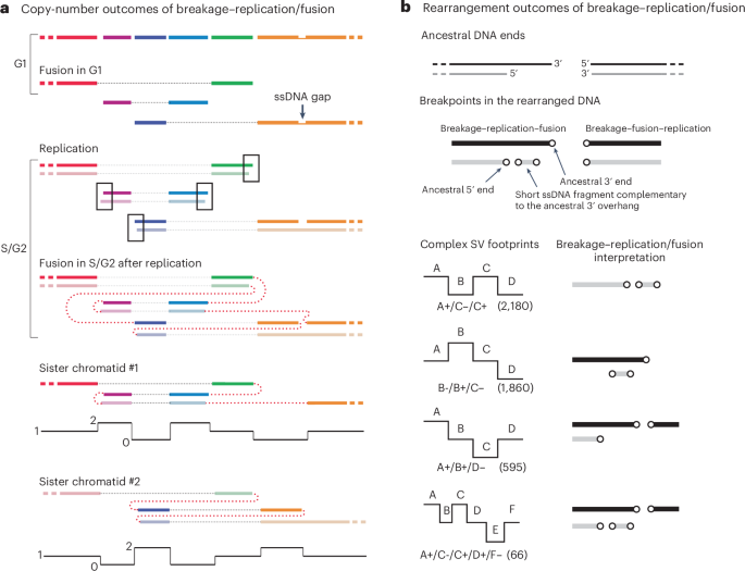
a, Segmental copy-number gain and loss generated by a breakage–replication/fusion cycle, including both breakage–fusion–replication and breakage–replication–fusion. The ancestral broken chromosome consists of six segments (shown in different colors) bounded by ten DSB ends; the rightmost segment also contains a single-strand gap with two ssDNA ends. Six DSB ends undergo ligation (fusion) in G1 (thin dotted lines), creating three chromosome fragments. After replication, there are seven new fragments (sister fragments are shown in dark and light colors) with ten new DSB ends: four pairs of sister DNA ends (outlined) plus two reciprocal DNA ends generated from the ssDNA gap. Fusions between the DSB ends in G2 (thick dotted lines) create reciprocal copy-number gains and losses on both sister chromatids. b, Footprints of rearrangement breakpoints generated by breakage–replication/fusion. Shown is one possible outcome when the left DNA end undergoes breakage–replication–fusion and the right DNA end undergoes breakage–fusion–replication. Top: ancestral DNA ends; middle: rearrangement breakpoints. Breakage–fusion–replication generates two flush breakpoints; breakage–replication–fusion generates two staggered breakpoints and a short insertion. Bottom: four complex structural variant (SV) footprints identified in cancer genomes16 that can be explained by breakpoints generated in one breakage–replication/fusion cycle. Each footprint is represented by a collection of breakpoints on either the left (−) or the right (+) of adjacent segments (A, B, …). Note that the breakpoint orientation (+/−) in the original study16 is opposite to our convention. The first three footprints (all having three breakpoints) were discussed in the supplementary information of the original study (pages 76–81); the last footprint with five breakpoints was shown in supplementary fig. 48 (page 82) of the same study. Numbers in parentheses represent the total counts of instances of each footprint reported in the original study, regardless of the joining pattern between breakpoints.