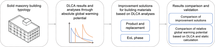
Figure 1 shows an overview of the methodological workflow of this study. We apply a DLCA approach to a solid masonry building typology using the dynamic environmental impact calculation, i.e., DLCIA. The results are analyzed from a temporal perspective to better understand the material characteristics. Subsequently, improvement solutions in both the product and End-of-Life (EoL) phases of building materials are modeled and evaluated using DLCIA to examine their effectivity of reducing the environmental impact. Herein, the improvement solutions in both the product and EoL phases also reflect the material replacements during the building operation. These improvement solutions are analyzed both individually and in combination to provide recommendations for achieving more sustainable building construction practices.
Data collection
In this study, we identify the materials in different building components of the solid masonry typology, based on the new construction building component catalog from a previous study44.The investigated building components include: base plate (BP), floor (FL), exterior wall (EW), flat roof (FRO) and window (WIN). For each building component, the materials are mapped with the activities from ecoinvent 3.11 (see supplementary material). Due to the data transparency and to enable the consistency of modeling, the study is conducted with data of the geographical context of Switzerland. The LCI values are then extracted from ecoinvent for use in the DLCIA calculation. As for the mass of each material, it is determined based on its properties, i.e., thickness, density, thermal conductivity, and the area of building components as derived from a case study building.
The investigated building is a campus facility constructed in 1968 on the main campus of the Technical University of Munich. In line with the nationwide non-residential building research project EnOB:dataNWG45, it is classified as a “Building for research and university teaching.” Based on the research in46, the original building age class was assigned to Group 1, constructed before 1918. Table 1 summarizes the original thermal transmittance (U-values) and values proposed for a new construction scenario, where the case study maintains the original geometry but adopts the modern standard.
A deep learning-based surrogate modeling approach was employed to evaluate the projected energy performance following the new construction in the case study. As a comparison, the energy performance of the status quo case is evaluated with the same approach. The energy model was trained on building energy simulation data generated through EnergyPlus for representative zones, as described in the authors’ previous work47. The geometry of these zones was derived using open data in the CityGML Level of Detail 2 (LoD2) format. From this data, the surface areas for the roof, ground, base, and shared wall surfaces were calculated, see Fig. 2. Specifically, the case study building has a BP of 4699 m(^2), FL of 15611 m(^2), EW of 3865 m(^2), FRO of 4699 m(^2) and WIN of 3104 m(^2). The window area was estimated based on assumptions from45. Based on the geometry and number of stories, the building was divided into distinct zones. Each zone identified from the LoD2 object was assigned four usage profiles: laboratories, group offices, lecture halls, and circulation areas based on own assumptions regarding the proportions of each type of usage and the research in EnOB:dataNWG45. The occupant behavior, heating schedules and the internal heat gains were then modeled according to the four representative profiles specified in DIN V 18599-1048. Subsequently, the net energy demand from the surrogate model is first converted to end-use energy using annual efficiency estimates from49, then to primary energy demand according to specific heating options per DIN V 18599-1048. The building originally relies on district heating from natural gas-powered heat and power co-generation (CHP). In the new construction, alternative heating options are evaluated.
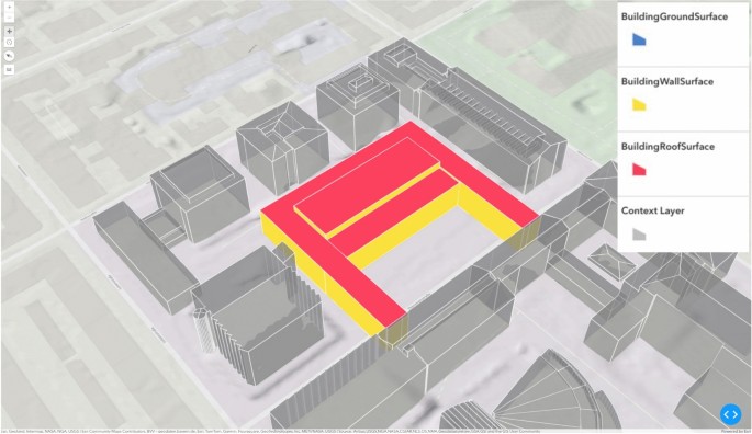
Illustration of the investigated building and the various construction parts.
DLCIA calculation
In the current LCA practices in the building industry, the GWP, expressed in kg CO(_2)-eq., is commonly used to indicate the environmental impact of different greenhouse gases relative to a reference gas, CO(_2), through the state-of-the-art life cycle impact assessment (LCIA) calculation. In general, GWP of each gas (i) is derived from its AGWP, as in Eq. (1). In this study, we use the AGWP based on the IPCC AR 650 to perform the DLCIA calculation.
$$begin{aligned} begin{aligned} textit{GWP}_i(H) = dfrac{{textit{AGWP}_i(H)}}{textit{AGWP}_{CO_2}} \ end{aligned} end{aligned}$$
(1)
where AGWP represents the integrated radiative forcing of each gas over time and is given in W m(^{-2}) year. It can be derived through Eq. (2):
$$begin{aligned} begin{aligned}&textit{AGWP}_i(H) = int _{0}^{H} textit{RF}_i(t) ,dt = int _{0}^{H} textit{RE}_{i}R_{i}(t) ,dt\&text {with} quad R_{i}(t) = exp (-dfrac{t}{tau _{i}}) end{aligned} end{aligned}$$
(2)
where (RE_{i}) is the constant radiative efficiency (RE), indicating the unit radiative forcing of each gas. (R_{i}(t)) represents the emission impulse remaining in the atmosphere over time and is expressed based on an exponential decay. Here, (tau _i) is the perturbation time scale of each gas.
In addition, the carbon cycle feedback is included in the calculation of AGWP and modeled differently for CO(_2) and non-CO(_2) gases. As in IPCC AR 5 and AR 643,50, the carbon cycle feedback of CO(_2) is modeled through a fitted (R_{i}), with the fitting parameters (tau _{i,n}) and (alpha _{i,n}) (Eq. 3), adopted from Joos et al.51.
$$begin{aligned} begin{aligned} R_{i}(t) = alpha _{i,0}+sum _{n=1}^{N}alpha _{i,n cdot }exp (-dfrac{t}{tau _{i,n}}) end{aligned} end{aligned}$$
(3)
As for the non-CO(_2) gases, the carbon cycle feedback is modeled through a nested convolution of climate-carbon feedback IRF (gamma R_{F}), AGWP and absolute global temperature potential (AGTP) (Eq. 4). The climate-carbon feedback instantaneous radiative forcing (IRF) (gamma R_{F}) is calculated through Eq. (5). The methodology and parametrization are based on Gasser et al.52. Subsequently, the (Delta AGWP) is treated as an additional value to be aggregated to the AGWP derived from Eq. (2).
$$begin{aligned} & begin{aligned} Delta textit{AGWP}_i(H) = int _{0}^{H} gamma R_{F}(H-t) int _{0}^{t} textit{AGTP}_{i}(tau ) cdot textit{AGWP}_{CO_2}(t-tau ) , dtau , dt end{aligned} end{aligned}$$
(4)
$$begin{aligned} & begin{aligned} gamma R_{F}(t) = gamma delta (t) – gamma (dfrac{alpha _1}{tau _1}exp (-dfrac{t}{tau 1})+dfrac{alpha _2}{tau _2}exp (-dfrac{t}{tau 2})+dfrac{alpha _3}{tau _3}exp (-dfrac{t}{tau 3})) end{aligned} end{aligned}$$
(5)
Here, AGTP is calculated through a convolution integral of the aforementioned IRF (R_{i}) of each gas. It is important to mention that (delta (t)) from Eq. (5) is a Dirac-(delta) function to approximate the CO(_2) flux at (t=)0. To practically model it and to reduce the computational cost in the calculation, we perform the calculation numerically, with a time stamp of 0.1 year. Accordingly, the Dirac-(delta) function (delta (t)) is approximated as 1 divided by the time stamp. The calculation method is applied to CO(_2), CH(_4), N(_2)O and 245 halogen gases, aligned with IPCC AR 650.
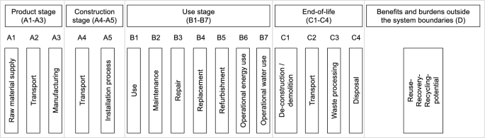
Life cycle phases of a building.
By using the dynamic AGWP obtained through the above method, the DLCIA calculation for the building is performed. Similar to that in the static LCA approach, different life cycle phases are considered according to EN 1597853, as shown in Fig. 3. The investigated life cycle phases in this study include product (A1–A3), replacement (B4), operational energy use (B6) and EoL (C). Accordingly, the basic calculation method can be expressed using Eq. (6):
$$begin{aligned} begin{aligned} EI = sum _{j=1}^{N}(m_{j,a}, , m_{j,b} ,, m_{j,c} ) cdot begin{pmatrix} textit{GWP}_{j,a}\ textit{GWP}_{j,b}\ textit{GWP}_{j,c}\ end{pmatrix} end{aligned} end{aligned}$$
(6)
where (EI) is the overall environmental impact of (N) investigated materials. (m_{j,x}) and ({GWP}_{j,x}) stand for the material mass and unit environmental impact aggregated for a certain period of time, e.g., 100 years as in (GWP_{100}), of each life cycle phase of each material. Herein, (a), (b) and (c) represent the product, use and EoL phases of the life cycle of each material, respectively. When applying the dynamic AGWP, Eq. (6) can be adopted and the material quantity (m_{j,x}) is transformed to (M_{j,x}) representing a set of various quantities subject to time. Accordingly, the calculation of each material’s embedded environmental impact is shown in Eq. (7):
$$begin{aligned} begin{aligned}&EI_j = (M_{j,a}, , M_{j,b4} , , M_{j,c} ) cdot begin{pmatrix} textit{AGWP}_{j,a}(RSP)\ textit{AGWP}_{j,b4}(RSP)\ textit{AGWP}_{j,c}(RSP)\ end{pmatrix}\&text {with}\&M_{j,a} = (m_{j,a}^{t=0 cdot RSL}, , …, m_{j,a}^{t=epsilon cdot RSL})\&M_{j,b4} = (m_{j,b4}^{t=0 cdot RSL}, , …, m_{j,b4}^{t=epsilon cdot RSL})\&M_{j,c} = (m_{j,c}^{t=1 cdot RSL}, , …, m_{j,c}^{t=epsilon cdot RSL})\&epsilon = RSP/RSL end{aligned} end{aligned}$$
(7)
where RSP is the reference study period and RSL represents the required service life of each material, i.e., life span of each material. (epsilon) is defined by RSP and RSL and represents the replacement frequency of a material in the use phase. Subsequently, with the RSL and (epsilon) of each material, the exact time point (t) for the material replacement can be defined. In this study, the RSP is 100 years, corresponding to the commonly applied (GWP_{100}) representing the GWP over 100 years after impulse. As aforementioned, instead of a single value, the material mass is given as (M_{j,x}) and the material quantity at specific time point is denoted as (m_{j,x}^{t}). It is to note that in case of having a linear supply chain based on the principle of cradle to grave, the material mass of replacement in the use phase B4, (M_{j,b4}), is identical as of the product phase (M_{j,a}). As a result, the DLCIA result is derived based on the mass of a material subject to time, obtained through the predefined construction typologies, and the AGWP of the material, defined through a multiplication of AGWP of each gas and the material-specific LCI extracted from ecoinvent.
As for the environmental impact during operation, ({EI}_{operation}), (m_{b6}) represents the annual primary energy demand as the life cycle stage B6 and the calculation is expressed by Eq. (8).
$$begin{aligned} begin{aligned} {EI}_{operation} = M_{b6} cdot {AGWP}_{b6} (RSP) ,,,text {with} ,,,M_{b6} = (m_{b6}^{t=0}, , …, m_{b6}^{t=RSP})\ end{aligned} end{aligned}$$
(8)
Using Eqs. (7) and (8) with both the cumulative and non-cumulative AGWP, we calculate both the integrated and temporal environmental impact of different materials, such that a comprehensive analysis for the building typology can be conducted.
DLCIA analysis
After conducting the DLCIA calculation, the environmental impact results can be shown and analyzed dynamically. In this study, both embedded and operational emissions are calculated and the results are analyzed on building, building component and building material levels, respectively. To gain a deep insight in the material characteristics, the analyses include the AGWP value, which shows the total environmental impact, along with the slope of non-cumulative AGWP over time and the dynamic share of different building components or materials that present the trend of emission impulse. Based on these analysis criteria that are either examined individually or in combination, the material characteristics can be further understood and improvement solutions can be potentially guided.
Modeling of improvement solutions
After the DLCIA analysis, different improvement solutions are modeled and evaluated. In this study, the improvement solutions primarily focus on the building materials. Specifically, the improvement solutions focus on the product and EoL phases, which also directly influences the results of material replacements by managing the waste from the replaced materials and integrating new materials. Improvement solutions in the product phase include: (1) reduction of material quantities, e.g., through lightweight construction with hollow structure; (2) use of alternative materials, e.g., alternative insulation materials. It is important to note that this study does not consider the impact of material changes on the U-values of the building envelope. The consequent influence on operational energy use was excluded to avoid conflating dynamic effects and to maintain a clear focus on the DLCIA of embodied emissions. As for the EoL phase, the improvement solutions are based on the future estimation of a higher circular recycling rate responding to the promoted concept of circular economy. In the current modeling strategy that mirrors the current recycling situation, deconstructed materials after their RSLs are usually fed into another product supply chain. Accordingly, the EoL and product phases of one material for replacement are usually separately calculated. This modeling strategy often results in a simple cut-off in the product phase and the neglect of the burdens occurring during the waste treatment when considering recycling measures. To address this, we model a circular recycling process that reintegrates the treated demolition waste after the material replacement into the production of virgin materials for the same product. For material replacement after the initial material reach its RSL, we assume that the replacement materials are also produced using the circularly recycled materials, following the same recycling strategy. Accordingly, the evaluation of one material not only considers the further treatment of demolition waste in the EoL phase to prepare for the circular recycling, but it also reduces the demand for virgin materials to produce the replacement material. As the waste treatment and replacement happen in the future, we identify the recycling rate for the relevant years dynamically to more accurately model this process. Specifically, an annual increase of the reduction in the virgin material of 1% is estimated based on the material reduction goal from the Swiss federal Circular Gap Report54. Based on this and by also considering the subtraction of waste materials throughout the supply chain that can be directly reused in the product phase without further treatment, an annual increase in the circular recycling rate is defined accordingly. Subsequently, the circular recycling rate and reduction rate in the virgin material at each replacement point are defined. Figure 4 shows the modeling principle of the circular recycling with the influences on the initial waste treatment process and the production process with virgin materials. Here, (gamma) stands for the circular recycling rate and (theta) represents the reduction in the virgin material subject to time.
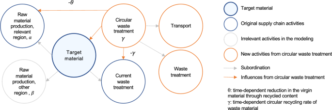
Modeling principle of the circular recycling.
The influences of the improvement solutions can be calculated using equation (7). For the improvement solutions in the product phase, the initial (M_{j,a}) and (M_{j,b4}) are changed by the material quantity reduction. The initial (AGWP_{j,a}) and (AGWP_{j,b4}) are replaced by alternative AGWP due to the use of alternative materials. Herein, the individual material mass (m_{j,a}^{t}) and (m_{j,b4}^{t}) remains identical due to the linear supply chain. As for the improvement solutions in the EoL phase, Eq. (7) is used for each raw material production or relevant component of each investigated target material. Specifically, the mass of the raw material production or relevant component at each replacement point, (m_{j,b4}^{t}), is not identical as (m_{j,a}^{t}) and is gradually reduced by the reduction rate (theta) of the circular recycling at each replacement point. Here, this reduction in the raw material is limited by its maximum portion in the investigated material, i.e., the reduction rate (theta) at any time point should not exceed the original portion of the raw material, (alpha). Accordingly, the circular recycling rate and the reduction rate remain constant after (theta) reaches (alpha). The material mass in the EoL phase is modeled similarly. (m_{j,c}^{t}) represents the quantity of either the initial waste treatment or the subsequent waste treatment necessary for the circular recycling, which are both determined by the circular recycling rate (gamma) at each replacement point (see Fig. 4). It is important to mention that the improvement solutions in the EoL phase do not influence the environmental impact at (t=0), since the solutions are future driven.
Cross-validation of GWP results: static versus dynamic calculation methodologies
To validate the DLCIA results, a comparative analysis was performed against the conventional static calculation. For better comparability, both methods were applied to calculate the GWP. Figure 5 shows a schematic representation of both methods applied to an example with a 30-year RSL. The conventional static approach uses a static characterization factor, i.e., (GWP_{100}), applied to each material production and replacement event, regardless of its temporal occurrence within the RSP. This method aggregates impacts from discrete events as if they were simultaneous, neglecting the temporal sequence of emissions. As a result, it fails to account for the continuous decay of the GHGs in the atmosphere and their continuous impacts, treating the impact of an emission at time (t=0) as identical to an emission at time (t=n). In contrast, the dynamic GWP calculation uses time-dependent characterization factors derived from the AGWP via the DLCIA calculation. This approach calculates the relative GWP at the exact time of each emission event, accurately reflecting the changing radiative forcing effect of GHGs throughout the whole period. The dynamic calculation is detailed in Algorithm 1, where the DLCIA approach is represented by the function “CalculateDynamicImpact” and “Timeshift” models the material replacements. The time horizon (TH) varies according to the exact time point of the emission event, as shown in Fig. 5. In addition, for a direct comparison with the existing literature38,40, a second dynamic calculation is performed using the DLCIA results and a fixed 100-year TH characterization factor.
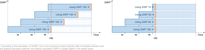
Schematic representation of GWP calculation using static and dynamic methodologies (left: static calculation, right: dynamic calculation).
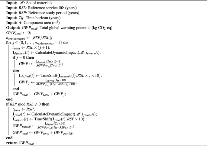
Algorithm of GWP calculation based on the AGWP results from the DLCIA calculation.