Insights in nonlinear ground response in volcanic environments from distributed dynamic strain sensing

Volcanic explosions catalogue & classification

During the three-month recording period (July 1 to September 24), we detected over 65,000 volcanic explosion over infrasound sensors (see Method: Detection of volcanic explosions) with common frequency content ranging from 0.7 to 4 Hz (Fig. 2a). We measured peak-to-peak (p-p) pressure and pressure rate for each event across all infrasound sensors, averaging the p-p values from all single infrasound sensors to obtain a single p-p value per acoustic event. p-p amplitudes between sensors do not present high variability, as their coefficient of variability is mostly below 0.1 (10%) for most of the events (Supplementary Fig. S1).

We identified two eruptive periods (A and B, Fig. 2a) happening at the time of recording, also in agreement with a previous study²⁰. The eruption periods are characterized by sudden increase in tremor RMS seismic amplitude and number of volcanic explosions per day (Fig. 2a). Notably, average p-p pressure and pressure rate values were higher during these periods (Fig. 2a).

We focus only on the eruptive period A, ranging from July 14 to July 22 (Fig. 2a; red box). Eruption period B (Fig. 2a; gray box) presents signal artifacts (saturation) in the DDSS²¹ produced by large amplitude (>100 Pa) volcanic explosions and infrasound tremor, which could interfere with the detection, classification and analysis of the GR events (see Methods and Supplementary Fig. S2). The DDSS dynamic range set during this study is about (3 cdot 10^{-5} s^{-1}) due to acquisition parameters²¹ (see Methods: Data acquisition). This translates to a p-p strain rate amplitude limit of (6 cdot 10^{-5} s^{-1}).

To investigate the GR, we analyse the interaction between a single type of acoustic pressure input (explosions) and the different resulting deformation outputs in the ground along the fibre path (GR signals in DDSS). To isolate different types of acoustic inputs, we classify the explosions based on waveform similarity (WS; see Methods: Classification of Volcanic Explosions), a robust and simple approach, also applied to infrasound signals at Mt. Etna^22,23. This classification method groups explosions into explosion families using the maximum cross-correlation (CC) value obtained between pair of events, and comparing it with a CC threshold (CC threshold of 0.88). The method also ensures that each explosion family contains at least two similar waveforms (see Methods: Classification of Volcanic Explosions)^24,25.

In total, we identified 111 volcanic explosion families. Fig. 2b displays the first thirteen explosion families, with templates shown in Fig. 2c. Some explosion families such as 10 and 13 exhibit two distinct explosions in their templates (Fig. 2c), which is a product of classifying explosion windows containing two pulses with an occurrence is less than 2 seconds.

The classification algorithm sorts families in descending order by the number of explosions they contain; thus, explosion families 1 to 5 comprise 5683, 479, 221, 147, and 84 explosions, respectively, making up 78% of the 8394 explosions in the eruptive period A. Explosion families 6 to 111 comprises 15% of the total and only near 7% (528 explosions) remain unclassified.

Two craters were active during the eruptive period A. Back-azimuth estimates from the infrasound array (Methods: Detection of volcanic explosions) indicate that the NSEC crater (Fig. 1) produced most of the explosion signals. Due to the azimuthal coverage of the network, craters NEC and BN, which were active at this period with NSEC²⁶, can not be differentiable. All explosion families are exclusively from NSEC, with exception of family 4, which could have its origin from BN, NEC and NSEC (Fig. 2b). Additionally, explosion signals from BN/NEC have generally less amplitude and longer periods than the ones coming from NSEC (Fig. 2b and 2c).

Ground response observations

We analyse the ground response (GR) signals recorded in the DDSS due to the energy coupling of the volcanic explosions infrasound waves into the near-surface. The observed GR events are high-frequency signals (10–50 Hz) of short duration ((<1) sec) recorded in the near-surface and linked to volcanic explosions. To build a GR event catalogue, a three-second window of DDSS data is selected, centred on the mean arrival time of the highest peak in the waveform associated with the explosion recorded across all infrasound stations (see Methods: Ground Response classification). Some GR event windows show clear GR signals across channels with 10–50 Hz frequency content, while others do not. For example, Fig. 3 compares the ground response differences between two volcanic explosions captured by the infrasound array. Both explosions originate from the New Southeast Crater (NSEC) and belong to the same explosion family (explosion family 1).

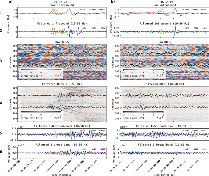
Two examples (a and b) of recorded volcanic explosions. The first row shows the raw infrasound signal recorded at three different infrasound sensors (ARB2, ARC2, ARD2). The second row shows the filtered signal between 10 and 50 Hz. The third row shows the corresponding GR event observed in raw DDSS data with two examples of DDSS signals at channels 420 and 650. The fourth row shows the same DDSS data of row third, filtered between 10 and 50 Hz. The fifth row is filtered (10 – 50 Hz) signals recorded on E-W component at three different broad-band seismometers. The sixth row shows the vertical (Z) component. The two explosions correspond to the same explosion family (explosion family 1), day (18-07-2019) and source (NSEC; back-azimuth estimations; see Methods: Detection of volcanic explosion). The explosion in a triggers a clear GR event, while in the explosion b the GR event is not clearly observable.

The first explosion example (Fig. 3a) shows an average peak-to-peak (p-p) pressure amplitude of 17 Pa, calculated from individual measurements across the infrasound array and filtered between 0.7 and 4 Hz. This explosion triggered a ground response above 10 Hz, observable in the unfiltered DDSS data (Fig. 3a, fourth row). The BB data also captured the ground response, observable with an applied 10–50 Hz band-pass filter (Fig. 3a, fifth row).

In contrast, the second explosion example (Fig. 3b) produced a p-p pressure amplitude of 3.4 Pa (filtered between 0.7 and 4 Hz), lower than the first explosion, but it did not generate a clearly observable ground response (Fig. 3b). However, in this case, the DDSS record indicates a possible ground response in a specific range of channels (700–800) compared to the other channels (Fig. 3b, fourth row). More examples of volcanic explosions can be seen in Supplementary Fig. S3 to S7, and associated GR events in Supplementary Fig. S7 to S10.

High-frequency content is also present in the explosion signals (Fig. 3). Filtered signals between 10 and 50 Hz (Fig. 3, second row) reveal emergent high-frequency waves occurring simultaneously with the primary low-frequency signal of the volcanic explosions (Fig. 3, first row).

Ground response classification

Each explosion might produce a resolvable GR signal at multiple channels. The produced GR signal could differ from channel to channel due to different variables, such as: cable segment orientation respect to craters, changes in the local near-surface properties (temporal and spatially), or amplitude of the explosion signal. Therefore, to find any unbiased relationship between explosions (taken as input; see Results: Volcanic explosions catalogue & classification) and the induced GR signals (taken as output), we classify the GR signals independently from the explosions.

To account for spatial and temporal variability of the GR signals, we modified the waveform similarity (WS) algorithm from the explosion classification (see Methods: Ground response classification) in order to relate GR waveforms, both temporally and spatially. The GR classification required two rounds: a temporal classification (along the time axis for each channel) and a spatial classification (across templates for each channel). We validate the GR classification method using constructed synthetic GR data to recreate the complexity of temporal and spatial variation in GR signals (see Methods: Ground Response (GR) classification).

Processing continuous DDSS data spanning entire days or weeks demands substantial computational resources due to the high temporal and spatial resolution of the recordings. Additionally, strain rate values on individual channels can vary significantly due to the strong influence of the local media²⁷. However, as part of the preprocessing routines, the used DDSS interrogator performs a spatial averaging over the channels covering a segment equal to the gauge length value (10 meters)²⁸. Therefore, we selected channels of the GR event windows every 10 meters (from channels 134 to 825) to limit the analysis to independent measurements per gauge length.

The GR event classification identified 717 GR families. Unlike the explosion classification, the final order of families in the GR classification is not necessarily ranked by the number of members due to the two-round clustering process. Approximately 92% of the total waveforms across all GR events and channels remained unclassified.

Fig. 4a shows the spatial (channels) and temporal (consecutive explosions) distribution of classified ground responses, with events becoming more frequent between explosion 1000 and 4500. Spatially, the number of GR families per channel (Fig. 4b) remains relatively constant across neighbouring channels, except where the fibre optic cable path changes, or at fault crossings (Fig. 4b) and connectors (e.g., Channel 560). Certain channels, such as those in ranges 302–380 and 613–735, display a higher number of classified GR events (Fig. 4c). Most of the GR families arise from explosions with high p-p pressure amplitude (Fig. 4d).

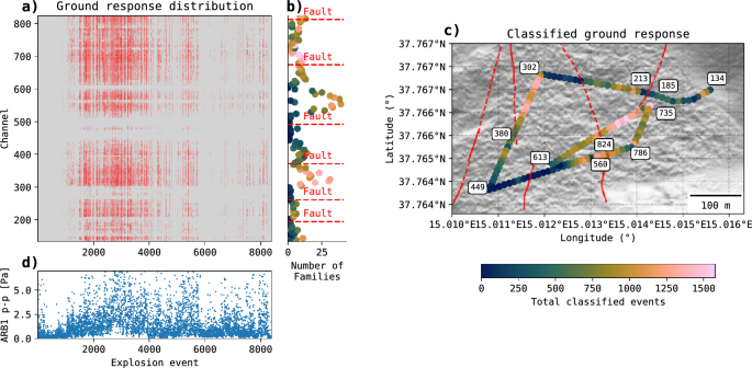
Obtained GR families from GR classification. a) Distribution of the obtained GR families across channels and for each explosion. Red colour represent classified GR event signals. Grey areas indicate GR event signals that were not classified (residuals). b) Number of GR families present at each channel. Fault crossed by the fibre optic cable are indicated in dashed red lines. c) Number of classified events per channel. Basemap done with Python and geospatial packages^45,47,48,49. d) peak-to-peak (p-p) amplitude of events captures at station ARB1.

The GR classification reveals that GR families are localized within specific sections of the fibre optic cable. Fig. 5a-m illustrate that GR families with the most members are concentrated in nearby channels within particular regions of the fibre path not spanning more than 50 m, with exception of GR family 4. Additionally, most of the GR waveform templates have a similar signature at the beginning of the wave, and discrepancies later in the coda train (Fig. 5n).

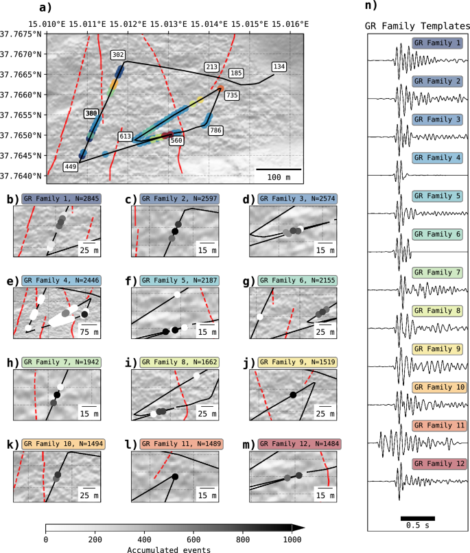
Spatial distribution of the first 12 GR families with the highest number of members. a) Overview map illustrating the presence of the first 12 GR families along the fibre optic cable (black curve) with distinctive colours for each GR family. Colours are connected to the labels of each GR family in subfigures b – m) and n). b – m) Zoomed view showing the local distribution of each GR family and their occurrence (number of accumulated events) at each channel where they are present, indicated by colour scale (lower part). n) Obtained waveform templates (normalized amplitude) from GR classification for each of the 12 GR families. Basemap done with Python and geospatial packages^45,47,48,49.

Strain rate and Pressure rate relation

The largest explosion family could induce more than one GR family from the ait-to-ground coupling. Therefore, we relate the peak-to-peak (p-p) pressure rate amplitudes from explosion family 1 measured in infrasound sensors with the p-p strain rate from the largest resulted GR signals measured in DDSS. The relation is observed for each GR family created by explosion family 1. Explosion family 1, being the biggest explosion family, represents already the 68% of the total amount of explosion events. Additionally, they are all originated from NSEC, and its members have the highest pressure amplitudes from eruption period A (Fig. 2b).

The GR classification distinguishes clear from unclear GR waveforms, ensuring only classified GR waveforms contribute to p-p strain rate values. This enables us to map GR event types within the possible elastic-mechanical states of the near-surface media.

In order to analyse the ground response per channel, Fig. 6 shows the relation between the p-p pressure rate from volcanic explosion of explosion family 1 and the strain rate amplitudes from the 12 biggest GR families previously shown in Fig. 5, at all channels. Each plot shows a linear fit (blue dashed curve) with a nonlinear fit as a third polynomial order. The nonlinear polynomial curve is divided into two or three segments, referred as elastic stages: Stage 1 (green), Stage 2 (orange) and Stage 3 (red). Each stage reports its (R^{2}) value for each of the elastic stages of the nonlinear curve (R2) in comparison to the linear fitting (R1). The (R^{2}) fitting score for a model between values (n le i le N) is calculated as:

where (y_{i}) is the real value i, (hat{y_{i}}) is the predicted value from the model, and (bar{y}) is the mean value.

In most of the cases, the R2 score is higher than R1, showing that nonlinear fitting describe better the data than the linear fitting. The denominator value in the slope (Young Modulus) of the linear fit is reported at each subplot, ranging from around 27 to 55 MPa. These range of values are in agreement with literature regarding unconsolidated granular material²⁹.

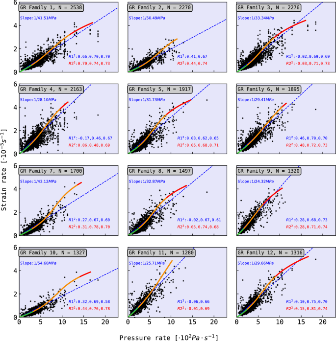
Strain rate of GR events with all channels associated to the GR families with the highest number of members vs. pressure rate of volcanic explosions from explosion family 1. Each plot presents a linear fitting curve (dashed blue line) and a 3rd order nonlinear curve (green-orange-red curve). The nonlinear curve represents the hyperleastic interpretation. The hyperplastic curve is composed by three stages: initial elastic behaviour (Stage 1: green curve), softening process (Stage 2: orange curve), and posterior stiffening (Stage 3; red curve). Each fitting curve has its (R^{2}) score reported: R1 for linear fitting, and R2 for nonlinear. For each elastic stage, there is an individual (R^{2}) score reported in order of the elastic stages.