Modeling strategies for a flexible estimation of the crude cumulative incidence in the context of long follow-ups: model choice and predictive ability evaluation | BMC Medical Research Methodology

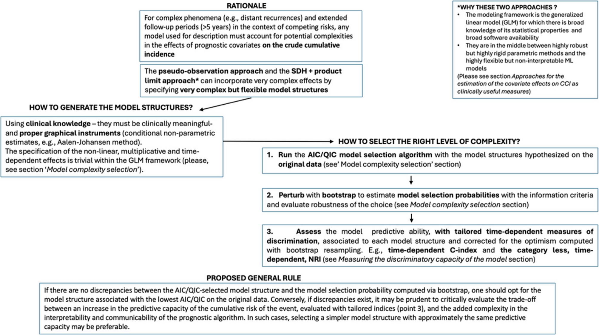
The proportionality of the SDH and the additivity of the effects are conditions that may not be satisfied in real applications, particularly in the presence of extended follow-up times and intricate biological phenomena. However, the design of randomized clinical trials and longitudinal cohort studies are under-powered to test complex interactions between covariates and/or time-dependent effects. In these cases, classical hypothesis tests fail or are impossible to apply when selecting the proper specification of the baseline function. This motivates the adoption of alternative criteria for the model selection task.

Information criteria like AIC and QIC (for the pseudo-likelihood of the GEE) represent a relevant approach. AIC quantifies the amount of information lost when a specific model is used to describe the real underlying process generating the data and is defined as:

Where (:K) is the number of model parameters and (:text{l}text{n}left(widehat{theta:};Xright)) is the log-likelihood function evaluated at the maximum likelihood estimates. The best model among a set of candidates is the one with the minimum value of the criterion. Therefore, AIC favors the goodness of fit of a model while penalizing over-fitted models with numerous parameters. It is important to note that AIC and AIC-like statistics are relative measures for comparing two or more models and indicate how closely a fitted model reflects the “true” data-generating process [32].

In the following section, we illustrate the detailed model selection strategy adopted in the current work. We considered a set of six regression models for distant recurrences, as shown below. The least complex model is a proportional hazards model with no interactions among covariates. The subsequent models introduce interaction effects of increasing complexity, including interactions between covariates and the baseline SDH function. The most complex effect consists of a second-order interaction between two covariates (nodal status and treatment) and the baseline SDH/risk function (Model 1). A second-order interaction refers to the combined effect of three variables on the response variable that cannot be explained by their individual effects or first-order interactions. Previous clinical knowledge, reflecting actual research hypotheses about tumor dormancy, motivates these patterns.

In the formulas below:

• (:Y) represents the discrete SDH or the risk for the pseudo-observations approach,

• (:varPsi:) is the vector of spline basis functions for the baseline time function,

• (:{X}_{T}) is the dummy variable for treatment (0 = surgical resection of the primary tumor by mastectomy, 1 = surgical resection by quartectomy),

• (:{X}_{N}) is the dummy variable for axillary nodal status (0 = node-negative, 1 = node-positive),

• (:otimes:) indicates the tensor product between the dummy variables and the spline bases. The tensor product term generalizes interactions by modeling the effect of two or more predictors as a product of basis functions for each predictor.

Model Specifications

1. 1.

   Model 1: A model with a second-order interaction effect between nodal status, treatment, and the baseline function. The model does not assume proportionality of the SDH or the risk function.

1. 1.

   Model 2: A model with an interaction effect between nodal status and the baseline function, an interaction effect between treatment and the baseline function, and an interaction effect between nodal status and treatment. The model does not assume proportionality of the SDH or the risk function.

1. 2.

   Model 3: A model with an interaction term between treatment and the baseline function, an interaction term between nodal status and treatment, and an additive effect of nodal status. The model assumes proportionality of the SDH or the risk function for nodal status but not for treatment.

1. 3.

   Model 4: A model with an interaction term between nodal status and the baseline function, an interaction term between nodal status and treatment, and an additive effect of treatment. The model assumes proportionality of the SDH or the risk function for treatment but not for nodal status.

1. 4.

   Model 5: A model with an interaction term between nodal status and treatment and an additive effect of treatment. The model assumes proportionality of the SDH or the risk function.

1. 5.

   Model 6: An additive model with no interaction effects. The model assumes proportionality of the SDH or the risk function.

Other than the time variable, the covariates used in the present work are all categorical. In cases where both categorical and numerical covariates are used, the following rules may be considered for specifying non-linear effects and interactions. The specification of non-linear effects or their interactions with a categorical variable follows the same approach illustrated above. Furthermore, the specification of interaction effects among numerical variables—including, as a special case, a time-dependent effect of a numerical covariate—may be obtained by employing a tensor product between the spline basis matrix for the baseline SDH or risk function and the spline basis matrix for the numerical covariate’s non-linear effect. A good example of the specification of a time-dependent effect of a numerical covariate (tumor size) on the CSH of the event can be found in [33].

The model selection procedure was as follows: we fitted each of the six models above several times with an increasing number of spline knots. We selected the optimal model according to the minimum QIC (in the direct approach) or AIC (in the indirect approach). We performed a perturbation of the data for assessing the robustness of the AIC-based selection, using sampling with replacement (i.e., non-parametric bootstrap). We compared the frequencies of the best model selected over 1,000 bootstrap samples with the model selected using the original sample.

Measuring the discriminatory capacity of the models

While the AIC provides valuable insights into which model best describes the real process underlying the incidence of an event of interest, clinical decision-making requires additional metrics. Specifically, when using a model as a tool for predicting patient outcomes, measures of model discrimination should complement information criteria. Here we show how these metrics might be useful in selecting a model for describing a phenomenon.

In most models, well-established prognostic factors are always included. The primary evaluation concerns whether incorporating complex terms—such as time-dependent effects or interactions between covariates—is necessary to predict better the absolute cumulative risk of an event. Both overall and time-dependent measures of accuracy are relevant. In the literature, several accuracy measures have been adapted from classical survival analysis to the context of competing risks. These include reclassification methods, the AUC, and prediction error curves.

Time-dependent C-index for competing risks in the discrete-time SDH and model on pseudo-observations

The C-statistic proposed by Harrell is widely recognized as a valid measure of discrimination and has been adapted for competing risks [22]. A key advantage of this measure is that it depends solely on the cumulative incidence function of an event.

A model with optimal discrimination ability, as measured by the time-dependent C-index, should maximize the concordance probability:

This measure can be evaluated at different follow-up time points. The inverse probability of censoring weighting (IPCW) methodology addresses the issue of censored observations when evaluating concordance, ensuring that (:{T}_{i}<{T}_{j}) even when (:j) corresponds to a censored observation.

Given that the present study focuses on estimating the C-index for cumulative incidence (CCI) using two different modeling frameworks, we employ the time-dependent C-index measure proposed by Wolbers. This measure is applied in the context of the discrete-time SDH model and the transformation model on pseudo-observations at 5 and 10 years of follow-up.

Time-dependent, category-less, Net Reclassification Improvement (NRI) for competing risks

For models containing standard risk factors and possessing reasonably good discrimination, a substantial “independent” association of the new marker (i.e., an added predictor increasing model complexity) with the outcome is necessary to achieve a significantly higher time-dependent C-index. Moreover, the C-statistic does not provide insights into the relative merits of alternative models for risk prediction.

The category-less NRI quantifies the improvement in discrimination achieved by incorporating an additional predictor (e.g., a new marker) into the model. Generally, an increase in discriminative ability arises from either an increase in the predicted probability of an event for subjects who experience it or a decrease in the predicted probability among those who remain event-free. The absolute NRI, adopted in this work, measures the proportion of subjects correctly reclassified—non-event subjects with decreased event probability and event subjects with increased event probability—among all subjects.

To complement this measure, we extend the concept of category-less NRI as a time-dependent metric for improved discrimination. The original formulation of the category-less NRI is:

Where (:{P}_{i,new}left(eventright)) and (:{P}_{i,old}left(eventright)) represent the predicted probabilities of an event from the new and old models, respectively, and (:{varDelta:}_{i}) is the event indicator (1 for an event, 0 otherwise).

In our setting, the absolute time-dependent category-less NRI is defined as:

Where (:{F}_{DR}^{new}left(t|{X}_{i}right)) represents the CCI function of DR up to time (:t) for subject (:i) with covariate values (:x), predicted with a model of increased complexity, and (:{F}_{DR}^{old}left(t|{X}_{i}right)) represents the CCI function of DR up to time (:t) predicted with the basic additive model. The term (:{varDelta:}_{i}=1left({T}_{i}, where (:{varepsilon}_{i}=1) defines the event of interest.

Thus, the category-less NRI in its time-dependent form assesses how effectively a new model, at time (:t), reclassifies subjects into higher or lower predicted risk categories relative to an old model, without relying on predefined risk categories. Instead, it focuses solely on whether an individual’s predicted risk increases or decreases correctly relative to the actual outcome.

Software

Software for augmenting the data matrix for each time interval and computing the interval-individual weights is already available in R as discSurv [34]. To generate pseudo-observations, we use the package pseudo [35]. GEE models were fitted using the package geepack [36].

Classical software to fit generalized linear models can be exploited to fit the models.

Illustration of the data

The “Milan 1” trial, held between June 1973 and May 1980, included 701 patients with unilateral breast cancer and no palpable axillary lymph nodes. Participants were randomly assigned to undergo a radical mastectomy (MAST) or breast-conserving surgery followed by radiotherapy (BCS + RT). In the BCS + RT group, complete axillary lymph node dissection was performed alongside BCS, followed by radiotherapy, with adjuvant chemotherapy introduced for node-positive patients starting in 1976. The trial results indicated no significant differences in disease-free or overall survival between the two groups, suggesting that BCS + RT was comparable to, if not better than, MAST.

In the “Milan 3” trial, conducted from December 1987 to December 1989, 567 eligible patients with breast tumors up to 2.5 cm in size were randomized to either BCS with or without immediate radiotherapy (RT). All patients underwent complete axillary lymph node dissection, with adjuvant therapy provided to those with node-positive disease, tailored according to menopausal status and tumor estrogen receptor (ER) status. The follow-up procedures mirrored those of the “Milan 1” trial. Initial results showed a reduced risk of local recurrence with RT following BCS, with no significant differences in overall survival between groups, except for patients with node-positive disease.