In order to compare the validity of various reasonable but ad hoc analytic approaches to the CCMAR-based estimators, we conduct a series of simulations. The aims of this simulation study are twofold:
-
1.
The primary goal of this simulation study is to learn where ad hoc approaches that combine imputation with some method to account for confounding can perform reasonably well, and where they may break down. Because the CCMAR-based IF estimator, (hat{chi }_a) has certain theoretical guarantees, benchmarking the performance of simpler approaches against the CCMAR-based estimators when data are generated under the factorization in Eq. (1) (e.g., when the nuisance models for CCMAR-based estimators are correctly specified) is of particular interest.
-
2.
A secondary goal of this simulation study is to evaluate the CCMAR-based estimators perform when data are generated by the alternative factorization in Eq. (3). In such settings, the performance of CCMAR-based estimators is more closely aligned with how such estimators are likely to fare in real world settings where component nuisance models are unknown to the analyst.
The framing of this simulation study is a hypothetical study comparing two bariatric surgery procedures on long term weight-loss maintenance [29]. Specifically, let A be a binary point exposure taking on value 0 for Roux-en-Y gastric bypass (RYGB) and 1 for vertical sleeve gastrectomy (VSG). We let Y denote the proportion weight Change at 5 years post surgery, relative to baseline. In our simulations we consider up to 5 confounders: gender, baseline BMI at surgery (centered at 30), an indicator of Hispanic ethnicity, baseline Charlson-Elixhauser comorbidity score [30], and an indicator of smoking status; we denote these confounders as (( L^{(1)}, L^{(2)}, L^{(3)}, L^{(4)}, L^{(5)} )), respectively.
To ensure our simulations reflect plausible real-world EHR-based settings, simulations are based on data from 5,693 patients who underwent either of the two bariatric procedures of interest at Kaiser Permanente Washington between January 1, 2008 and December 31, 2010. Complete information on gender, baseline BMI, and ethnicity, was available for all patients, while comorbidity scores were only available for 4,344 patients. Smoking status was not measured at all in the data, so we synthetically generated this confounder subject to partial missingness. This was done to create more complex scenarios with multiple partially missing confounders. In all simulation settings, the completely observed confounders were (L_c = ( L^{(1)}, L^{(2)}, L^{(3)})), while the partially observed confounders were either the univariate (L_p=L^{(4)}), or the bivariate (L_p = ( L^{(4)}, L^{(5)})), depending on the simulation setting.
Data generation process
A critical component of our simulation infrastructure is the specification of the “true” components of the likelihood factorization corresponding to each respective aim. There is a subtle but important relationship between which factorization is used as the data generating process (DGP) and the series of nuisance functions required for each estimator. In particular, the nuisance functions required by the CCMAR-based estimators directly align with those under the factorization in Eq. (1) and the nuisance functions required by other ad-hoc estimators align with those under the factorization in Eq. (3). When models required by each respective estimator align with components of the underlying DGP, it is straightforward to assess whether models are correctly specified because the “true” likelihood components are known. Similarly, when nuisance models required for an estimator do not directly correspond with likelihood components used to generate simulated data, it is not clear the degree to which component models may or may not be misspecified.
The choice of which factorization to use as the DGP in each scenario was thus driven by which aim the scenario hoped to evaluate. Scenarios targeting aim 1 generated data from the novel factorization expressed in Eq. (1), using CCMAR-based estimators using the “true” parametric models as a benchmark to compare a suite of approaches described in Methods section. Data generation under this factorization is described in Factorization in Eq. (1) section. Scenarios targeting aim 2 compared estimators on data generated from the alternative factorization of the coarsened observed data likelihood in Eq. (3), described in detail in Alternative factorization section and shown visually in Fig. 2b. In such scenarios, the “true” nuisance functions in the factorization proposed by Levis et al. [6] (i.e., those in Table 2) were unknown and would not necessarily be derivable in closed form. As such, results of simulations under this specification can help demonstrate how the CCMAR-based estimators might perform when the true underlying nuisance functions are unknown. This, of course, is akin to the problem faced by an analyst in any practical setting.
To inform specification of the “true” likelihood components for each factorization, a series of parametric models was fit to the Kaiser Permanente data as described in Factorization in Eq. (1) and Alternative factorization sections. This plasmode simulation set-up ensured that our set-up reflects the complexity of real EHR data to the extent possible by preserving complex correlation structures [31].In each simulation setting, 5,000 datasets of size (n = 4,344) patients were generated and analyzed according to the procedures outlined in the remainder of this section. In the main paper we present results from 4 data-driven simulations settings, summarized as follows.
-
1.
Factorization in Eq. (1), 1 partially missing confounder.
-
2.
Factorization in Eq. (1), 1 partially missing confounder, additional non-linearities and interactions in imputation mean model, induced skew in distribution of imputation model.
-
3.
Factorization in Eq. (1), 2 partially missing confounders, amplified interactions between (A, L_{p}), and Y in joint imputation model, induced skew in distribution of imputation model.
-
4.
Alternative factorization, 2 partially missing confounders, amplified interactions between (L_{c}, L_{p}) in full treatment model (tilde{eta }(L_c, L_p, a)).
Data-driven simulation settings 1-3 target aim 1, while setting 4 targets aim 2. Results from an additional 15 data-driven simulation settings targeting both aims (and generating simulated data from both factorization) are available in the Supplementary Materials.
Factorization in Eq. (1)
To inform simulated datasets under Eq. (1), each of the 4 nuisance functions for this factorization of the coarsened observed data likelihood, outlined in Table 2, were modeled by fitting regressions to the Kaiser Permanente data. These models were used to help specify the “true” components of the likelihood. Specifically, logistic regressions were fit for (eta) and (pi), and a Gaussian linear model was fit for (mu). In the Kaiser Permanente data, the comorbidity score ((L^{(4)} = L_{p1})) is categorical, but we instead chose to fit a generalized linear model with gamma link function to make the underlying relationship more complex. In fact, numerical integration techniques such as Gaussian quadrature are required to compute (hat{chi }_a) when (L_p) contains continuous confounders.
In certain simulation settings, we simulated a second missing confounder, smoking status ((L^{(5)} = L_{p2})) from a logistic regression model with pre-specified effect sizes given that no such smoker indicator is available in the Kaiser Permanente data. Such generation follows from the decomposition of the joint density of (L_p) as follows
$$begin{aligned}& lambda (ell _{p1}, ell _{p2} | L_c, A, Y, S = 1) = \&lambda _1(ell _{p1} | L_c, A, Y, S = 1)\&lambda _2(ell _{p2} | L_c, A, Y, S = 1, L_{p1} = ell _{p1}) end{aligned}$$
(4)
where (lambda _1) and (lambda _2) represent the conditional densities of the 2 confounders in (L_p), corresponding to (L^{(4)}) and (L^{(5)}), respectively.
In each simulation, (L_{c,1}…L_{c,n}) were drawn with replacement from the empirical values in the Kaiser Permanente data. Then, ((A_i, Y_i, S_i, S_iL_{p,i})) for (i = 1, …, n) were independently sampled, sequentially, from the following models, with covariates (X) and coefficients ((beta)) for each model simulations available in Table 3.
-
(text {logit}(eta (L_c, 1)) = text {logit}(P[A = 1 | L_c]) =)(beta _eta ^T X_eta)
-
(Y | L_c, A sim mathcal {N}(beta _mu ^T X_mu , sigma ^2_Y))
-
(text {logit}(pi (L_c, A, Y)) = text {logit}(P[S = 1 | L_c, A, Y]) =)(beta _pi ^T X_pi)
-
(L_{p1} | L_c, A, Y, S = 1 sim)(text {Gamma}(alpha , lambda _1(L_c, A, Y))) with rate parameter (lambda _1(L_c, A, Y))(= frac{alpha }{mathbb {E}[L_{p1} | L_c, A, Y, S = 1]}), and we parameterize (log (mathbb {E}[L_{p1} | L_c, A, Y, S = 1]))(= beta _{lambda _1}^T X_{lambda _{1}})
-
(text {logit}(lambda _2(L_c, L_{p1}, A, Y, S = 1)) =)(text {logit}(P[L_{p2} = 1 | L_c, L_{p1}, A, Y, S = 1]))(= beta _{lambda _2}^T X_{lambda _2}) (for simulations with multiple partially missing confounders).
We considered several settings where certain effects in the 4 nuisance models were amplified in order to create more interesting and complex relationships across confounders, treatment and outcome.
Alternative factorization
For aim 2, in order to asses the performance of CCMAR-based estimators where the “true” nuisance functions are unknown (and perhaps not derivable in closed form), we considered an additional data generating process based on Eq. (3) which reflects the more “natural” order described in the previous section. In simulations with multiple missing confounders, the joint density of (L_p) decomposes as follows:
$$begin{aligned} tilde{lambda }(ell _{p1}, ell _{p2} | L_c) =tilde{lambda }_1(ell _{p1} | L_c, )tilde{lambda }_2(ell _{p2} | L_c, L_{p1} = ell _{p1}) end{aligned}$$
(5)
where (tilde{lambda }_1) and (tilde{lambda }_2) represent the conditional densities of the 2 confounders in (L_p), corresponding to (L^{(4)}) and (L^{(5)}), respectively.
Similar to the data-driven strategy described in Factorization in Eq. (1) section, in order to simulate datasets under Eq. (3), each of the 4 nuisance functions for the alternative factorization of the coarsened observed data likelihood were fit to the Kaiser Permanente data to specify the “true” components of the likelihood. In fact, the type of parametric models used to fit these nuisance models under the alternative factorization were the same as under the previous factorization: logistic regressions were fit for (tilde{eta }) and (pi), a Gaussian linear model was fit for (tilde{mu }), a generalized linear model with gamma link function for (tilde{lambda }_1) and a logistic regression for (tilde{lambda }_2). The key differences between the models used to inform the truth in the previous factorization versus the alternative factorization are the sets of variables included in the relevant conditioning sets, i.e., what covariates can be conditioned on.
In each simulation, (L_{c,1}…L_{c,n}) were drawn with replacement from the empirical values from the Kaiser Permanente data. Then ((L_{p,i}, A_i, Y_i, S_i)) for (i = 1, …, n) were independently sampled, sequentially, from the following models.
-
(L_{p1} | L_c sim text {Gamma}(alpha , lambda _1(L_c))) with rate parameter (lambda _1(L_c) = frac{alpha }{mathbb {E}[L_{p1} | L_c]}), and we parameterize (log (mathbb {E}[L_{p1} | L_c]) = beta _{lambda _1}^T X_{lambda _{1}})
-
(text {logit}(lambda _2(L_c, L_{p1})) = text {logit}(P[L_{p2} = 1 | L_c, L_{p1}]))(= beta _{lambda _2}^T X_{lambda _2}) (for simulations with multiple partially missing confounders).
-
(text {logit}(eta (L_c, L_p, 1)) = text {logit}(P[A = 1 | L_c, L_p]))(= beta _eta ^T X_eta)
-
(Y | L_c, L_p, A sim mathcal {N}(beta _mu ^T X_mu , sigma ^2_Y))
-
(text {logit}(pi (L_c, A, Y)) = text {logit}(P[S = 1 | L_c, A, Y]))(= beta _pi ^T X_pi)
Even though S was generated after (L_p), the model used to generate S only conditions on (L_c, A, Y), and thus the CCMAR assumption in Eq. (2) is not violated. Because (L_p) was sampled before S in the above procedure, simulated values for (L_p) were set to be missing among patients sampled to be non-complete cases ((S = 0)), thereby ensuring analysis took place on the same coarsened observed data structure ((L_c, A, Y, L_p, SL_p)) as data generated under Eq. 1.
We considered several settings where certain effects in the 4 nuisance models were amplified in order to create more interesting and complex relationships across confounders, treatment and outcome. Covariates (X) and coefficients ((beta)) for each model are presented in Table 3.
Summary of scenarios
Because of differences in the relative ordering of component models between the two factorizations, coefficients in Table 3 are not directly comparable across scenarios using different factorizations. As such, we provide some additional summary information describing the four simulation scenarios.
The true average treatment effects, reflecting the relative (%) weight loss advantage of RYGB over VSG were 11.9%, 10.4%, 10.2% and 22.7%, respectively. Additional details on how these ground truth ATEs were computed is summarized in the Supplementary Materials (Section S4). The marginal probability of missingness, (p(S = 0)), remained fairly consistent across scenarios 1-4, totaling 32.5%, 30.8%, 30.8%, and 29.5%, respectively.
Unfortunately, we are unable to provide a single summary measure quantifying the magnitude of confounding directly attributable to (L_p), as that is a complex function of the distribution of observed (L_p), the strength of associations between (L_p, A) and Y, and the functional form of (L_p) in component nuisance models. Nevertheless, based on the dimension of (L_p) and magnitude of coefficients in Table 3, it’s reasonable to characterize the four simulation scenarios as increasing in terms of the complexity required to account for confounding due to (L_p) (scenario 1 easiest (rightarrow) scenario 4 hardest).
Methods
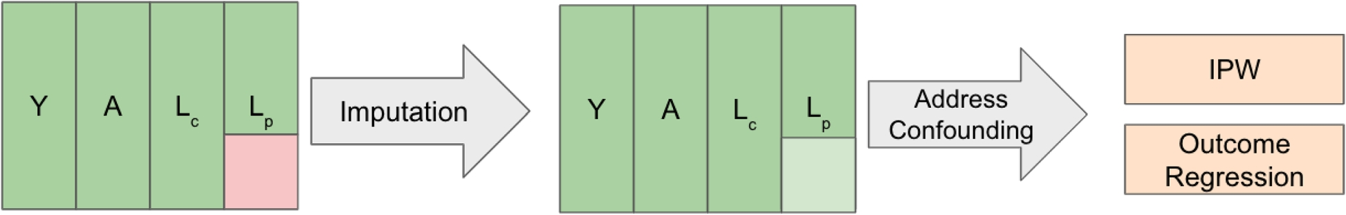
Across our simulation settings, we considered combinations of several methods for imputation of (L_p) in conjunction with the use of outcome regression or inverse probability weighting to address the issue of confounding. Specifically, we considered methods that vary in both model flexibility (parametric, semi-parametric, non-parametric) and structure (interactions vs. no interactions). Taken collectivity, the range of methods considered reflects the types of models analysts might used in practice [4], and as such serves as a useful set to evaluate in aim 1.
Under each imputation strategy, a parametric model was estimated for (L_p), and subsequently a single draw was sampled from the induced conditional distribution for each missing observation. The choice to use single imputation rather than multiple imputation helped ease computational given the large number of simulation scenarios and comparator methods considered. Three imputation models for (L_p) were considered: the correctly specified DGP for (L_p) (a gamma generalized linear model for comorbidity score ((L^{(4)})) and a logistic regression for smoking status ((L^{(5)})), with exact models depending on the corresponding factorization under which data were generated); a simpler imputation model with a Gaussian linear model for comorbidity score and a logistic regression for smoking status, with neither model considering any interactions; and, an imputation model with a Gaussian linear model for comorbidity score and a logistic regression for smoking status, while specifying all pairwise interactions. To avoid overfitting/variance inflation due to specifying all pairwise interactions, linear/logistic regression models in this third case were fit using glmnet [32] in R with (L_1) (LASSO) [33] regularization. Additionally, we considered a fourth strategy where the problem of missing data was ignored and subjects with missing these data were dropped, in order to mimic a complete case analysis.
Upon imputing (or not imputing) (L_p), we considered several methods to directly model Y in order to estimate the mean counterfactual outcome (mathbb {E}[Y^{(a)}]) using outcome regression. In particular, we considered 3 types of models ranging in flexibility: linear regression, with no interactions and with all pairwise interactions specified; generalized additive models (GAMs) [34], with no interactions and with all pairwise interactions specified; and random forest. As was the case with the linear regression models used for imputation of (L_p), outcome regression models specifying all pairwise interactions were estimated with (texttt {glmnet}) [32] using (L_1) (LASSO) [33] regularization.
In the case of GAMs, interactions took on one of three forms. When two covariates were binary, interaction effects were simply the coefficient for product of the covariates, as in a linear regression model. For covariates (x_1 in {0, 1}, x_2 in mathbb {R}), interaction effects were the coefficients for the product (x_1f(x_2)), where f is some smooth basis function. Finally, when both covariates were continuous, interaction effects were coefficients for the two dimensional surface (g(x_1, x_2)). In our fitting of GAMs, f was chosen to be a cubic regression spline, while g was a tensor product smoother. Inherent to the fitting of these smooth functions is regularization in the form of choice of degree and/or knots [35]. Finally, we considered an even more flexible non-parametric random forest model, which can capture complex, highly non-linear relationships between confounders, treatment and outcome.
We employed a similar suite of approaches for IPW as we did for outcome regression, instead modeling the probability of treatment using several models varying in complexity and flexibility. The analogue of the linear regression (with and without interaction effects) when modeling propensity scores was logistic regression, while GAMs with logit link (i.e., GAM logistic regression) were used as the analogue of GAM outcome regression. Random forests were also applied under classification specification to most flexibly model the treatment mechanism. Table 4 summarizes the suite of “standard” models.
Consistent with aim 1, CCMAR-based estimators were computed using correctly specified parametric models in scenarios where data was generated under Eq. (1) (scenarios 1–3). Towards evaluation of aim 2, we fit three versions of the CCMAR-based estimators in scenarios where data was generated under Eq. (3) (scenario 4). First, we fit the same parametric models used in scenarios 1-3, which we anticipate would be misspecificed. Given that the induced form of the correct nuisance functions under Eq. (1) was not easily derived in closed form when data were generated under Eq. (3), we considered a flexible version of the CCMAR-based estimators leveraging GAMs with logit link for (hat{eta }), (hat{pi }) and (hat{lambda }_2), a traditional GAM for (hat{mu }), and a GAM with underlying gamma distribution for (hat{lambda }_1). In this flexible version of the CCMAR-based estimators, GAMs include all pairwise interactions. We also considered a flexible version of the CCMAR-based estimators with a GAM with underlying Gaussian distribution for (hat{lambda }_1).