Mechanical testing
Tensile strength and young’s modulus
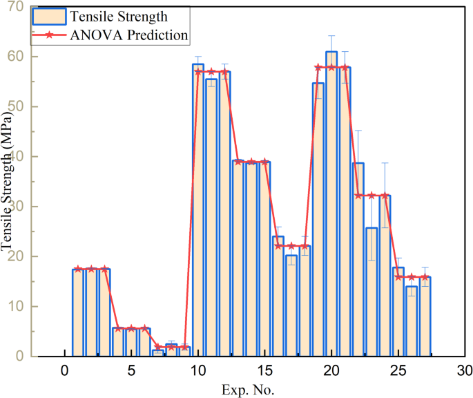
The tensile strength and Young’s modulus of PLA/CCB composites were evaluated using an L27 orthogonal array designed through the Design of Experiments (DOE) approach, as shown in Table 2. Figure 3 presents the variations across experiments 1 to 27. The minimum tensile strength was observed at Experiments 7–9 with 1.27–2.5 MPa for pure PLA. Similarly, experiments 19–21 exhibit a maximum tensile strength of 54.6-60.99 MPa for 10 wt% PLA/CCB composites. A similar trend was observed for Young’s modulus; experiments 25–27 and 19–21 exhibit a minimal of 105–110 MPa and a maximum of 2652–3561, respectively. These findings demonstrate that both tensile strength and Young’s modulus of PLA/CCB composites are significantly enhanced by increasing the CCB filler content and optimizing the processing conditions, particularly temperature, injection speed, and pressure.
Tensile strength and Young’s modulus vs. experiment number.
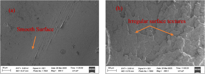
Fractography of (a) Pure PLA; (b) 10 wt% PLA/CCB composite.
Figure 4a and b illustrates the fractured surface morphology of pure PLA and PLA/CCB composites after tensile test, revealing differences in their failure behavior. Figure 4a shows the fracture surface of pure PLA, which appears smooth, continuous, and homogeneous, characteristic of a relatively ductile fracture48. In contrast, Fig. 4b displays the fractured surface of the PLA composite reinforced with 10 wt% CCB, exhibiting a rough, irregular texture with visible surface discontinuities. Incorporating rigid biochar particles disrupts the matrix continuity, creating localized stress concentrations that promote crack initiation and propagation, which is characterized by brittle fracture behaviour49.
Hardness testing
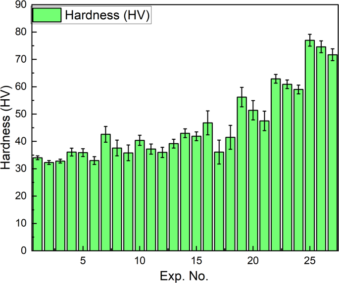
Figure 5 illustrates the hardness of the PLA/CCB composites. Experiments 1–3 exhibit minimal hardness, ranging from 32.3 to 34 HV for pure PLA. However, the experiments 25–27 showed maximum hardness of 71.7 to 77 HV for composites with 10 wt% CCB. These findings clearly demonstrate that increasing the CCB content along with optimizing the processing conditions significantly enhances the hardness of the PLA/CCB composites.
Statistical analysis
Taguchi analysis
The experimentally obtained values of tensile strength, Young’s modulus, and hardness were used to calculate the corresponding signal-to-noise (S/N) ratios for the Taguchi analysis, as presented in Tables 2 and 3. The following sections discuss the optimization of the significant process parameters for each response variable based on the Taguchi method.
Tensile strength
Tables 4 and 5 summarize the influence of varying process parameters on tensile strength, considering both the mean values and the larger-is-better signal-to-noise (S/N) ratio. The analysis reveals that composition is the most significant parameter, with the highest delta values of 16.47 and 31.02 for the mean and S/N ratio, respectively. Temperature follows as the second most influential parameter, with delta values of 13.32 and 30.821. In contrast, injection pressure with 3.72 and 6.245 and injection speed with 3.31 and 8.961 exhibit relatively lower delta values for both metrics, indicating a minimal effect on tensile strength. This analysis demonstrated that increasing filler content (composition) and processing temperature have a substantial positive impact on the tensile strength of the composites, while variation in injection pressure and speed has minimal effect.
Figures 6a and 7a present the main effects plots for tensile strength based on the signal-to-noise (S/N) ratio and mean values, respectively. Both plots clearly demonstrate that composition and temperature are the most influential factors affecting tensile strength. From the graphs, it is evident that tensile strength significantly improves as the composition increases from neat PLA to 5% CCB. However, beyond this point, the improvement stabilizes. In the case of temperature, a decline in tensile strength is observed as the processing temperature increases from 135 °C to 155 °C. Additionally, injection pressure and injection speed exhibit moderate effects, displaying nonlinear behavior. In the S/N ratio plot, an increase in injection speed and a reduction in injection pressure lead to a decrease in tensile strength. In contrast, the mean response plot shows an opposite trend, where increasing both injection pressure and injection speed slightly enhances tensile strength. Overall, composition and temperature are confirmed as the most dominant parameters influencing tensile strength, while injection pressure and injection speed have comparatively lesser effects.
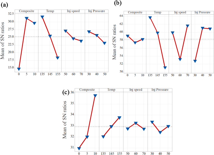
Mean of S/N ratio for (a) tensile strength; (b) Young’s modulus; (c) hardness.
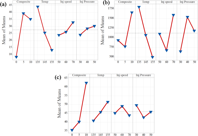
Mean of means for (a) tensile strength; (b) Young’s modulus; (c) hardness.
Young’s modulus
Tables 6 and 7 present the influence of process parameters on Young’s modulus, considering both the mean values and the larger-is-better signal-to-noise (S/N) ratio. The analysis indicates that temperature is the most significant factor affecting Young’s modulus, as reflected by its highest delta values of 12.57 for the S/N ratio and 1300 for the mean. Following this, injection speed, injection pressure, and composition show progressively lower influences, with delta values of 8.43 and 918.9, 8.26 and 894.9, and 1.72 and 885.0, respectively. These results suggest that increasing the processing temperature substantially enhances Young’s modulus, while the effects of injection speed, pressure, and composition are comparatively less pronounced.
The main effects plots for both the signal-to-noise (S/N) ratio and mean values of Young’s modulus are presented in Figs. 6b and 7b. These plots demonstrate that temperature is the most influential factor among all process parameters. Both the S/N ratio and mean response attain their highest values at 135 °C, indicating that this temperature level provides the most robust performance, reinforcing its dominant effect on Young’s modulus. Injection speed emerges as the second most significant factor, with both plots identifying 50 mm/s as the optimal level for achieving better robustness. However, the slightly lower mean response at this setting suggests a trade-off between performance consistency and modulus value. Composite content also contributes notably, where 5% CCB content offers better robustness, while 10% CCB yields the highest mean modulus. Injection pressure, on the other hand, shows the least influence, with minimal variation across different levels, although 40 MPa demonstrates a marginally better performance.
Hardness
The hardness of PLA/CCB composites under different processing parameters was evaluated using the signal-to-noise (S/N) ratio and mean values, as summarized in Tables 8 and 9. The analysis indicates that composition is the most influential factor, with the highest delta values of 4.80 for the S/N ratio and 26.79 for the mean ranked as 1. Temperature is the second most significant factor, exhibiting delta values of 1.73 (S/N ratio) and 10.66 (mean). Injection pressure ranks third, with delta values of 0.95 (S/N ratio) and 6.89 (mean), while injection speed shows the least influence, with the lowest delta values of 0.54 (S/N ratio) and 5.19 (mean). Overall, this summary demonstrates that composition has the most dominant effect on enhancing the hardness of PLA/CCB composites, whereas injection speed contributes minimally, highlighting the dominant role of filler content and processing temperature in enhancing the mechanical performance of PLA/CCB composites.
Figures 6c and 7c present the main effects plots for both the signal-to-noise (S/N) ratio and mean values, illustrating the influence of process parameters on the hardness of PLA/CCB composites. These plots show that an increase in composition has the most significant effect on hardness. Temperature and injection pressure show a moderate influence, while injection speed has the least effect. This trend indicates that composition is the dominant factor governing hardness, followed by temperature, injection pressure, and injection speed. The consistent patterns observed in both the S/N ratio and mean response plots further confirm the reliability and validity of this analysis.
Analysis of variance (ANOVA)
Tensile testing
The ANOVA results presented in Table 10 indicate that the injection molding process parameters statistically affect the tensile strength of PLA/CCB composites, as evidenced by a P-value of 0.000 (P < 0.001). This confirms a highly significant influence of the selected process parameters and composition on tensile strength. Among these, composition and temperature were the most impactful factors, contributing 50.43% and 42.67%, respectively. In comparison, injection speed and injection pressure contributed relatively less, at 3.86% and 1.82%, respectively. The remaining 1.22% was attributed to experimental error, suggesting excellent process control and repeatability. Additionally, the regression analysis demonstrated a strong correlation between tensile strength and the process parameters. The model showed a high goodness of fit, with a coefficient of determination (R2) of 98.78% and an adjusted R2 of 98.23%, indicating the model’s high accuracy, reliability, and suitability for predicting tensile strength outcomes based on the chosen parameters.
Regression Eq.
$$begin{gathered} {text{TS}},=,{text{27}}.{text{664}}, – ,{text{19}}.{text{338}}{{text{F}}_{text{1}}}+{text{11}}.{text{686}}{{text{F}}_{text{2}}}+{text{7}}.{text{652}}{{text{F}}_{text{3}}}+{text{16}}.{text{452}}{{text{T}}_{text{1}}} hfill \ – {text{2}}.0{text{83}}{{text{T}}_{text{2}}} – {text{14}}.{text{369}}{{text{T}}_{text{3}}} – {text{3}}.{text{731}}{{text{S}}_{text{1}}} – {text{1}}.{text{499}}{{text{S}}_{text{2}}} hfill \ +{text{5}}.{text{23}}0{{text{S}}_{text{3}}} – {text{3}}.{text{548}}{{text{P}}_{text{1}}}+0.{text{85}}0{{text{P}}_{text{2}}}+{text{2}}.{text{697}}{{text{P}}_{text{3}}} hfill \ end{gathered}$$
(22)
Here, F1, F2, F3: Composite levels (0%, 5%, 10%), T1, T2, T3: Temperature levels (135 °C, 145 °C, 155 °C), S1, S2, S3: Injection speed levels (50, 60, 70 mm/s), P1, P2, P3: Injection pressure levels (30, 40, 50 bar), and TS: Tensile Strength (MPa).
Tensile strength prediction accuracy based on ANOVA model.
Figure 8 presents a comparison between the experimentally measured tensile strength values and those predicted using the ANOVA-based regression equation (Eq. 22). The comparison reveals that most of the experimental values fall within a 10% error margin, indicating strong agreement between the experimental results and the model predictions. For instance, tensile strength values around 17.5 MPa show minimal deviations of approximately ± 0.57%, while values near 5.6 MPa and 22.1 MPa have percentage errors of ± 2.41% and ± 8.6%, respectively. Similarly, measurements close to 38.95 MPa and 57 MPa exhibit even smaller errors of around ± 0.13% and ± 1.5%, confirming the high accuracy of the model.
However, a few data points show larger deviations. Tensile strengths near 15.9 MPa and 32.2 MPa exhibit higher percentage errors of ± 11.95% and ± 20.19%, respectively, slightly exceeding the 10% threshold and suggesting the need for further investigation. The largest deviation is observed for a value near 1.9 MPa, with an error of approximately ± 32.63%. Despite these few outliers, the majority of the data points demonstrate excellent predictive accuracy, underscoring the robustness and reliability of the regression model in capturing the influence of processing parameters on tensile strength.
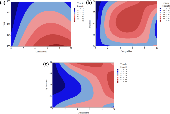
Contour plot analysis for tensile strength on (a) composition and temperature; (b) composition and injection speed; (c) composition and injection pressure.
The contour plots presented in Fig. 9 illustrate the combined effects of two process parameters on the tensile strength of PLA/CCB composites, while keeping the other parameters constant. In Fig. 9a, the interaction between composition and temperature reveals that higher tensile strength values (above 60 MPa, shown in red) are achieved when the composition ranges between 4% and 8% and the processing temperature lies between 135 °C and 145 °C. Conversely, lower tensile strength values (below 30 MPa), represented by blue regions, occur at low filler content combined with higher temperatures. Figure 9b depicts the interaction between composition and injection speed, showing that maximum tensile strength is obtained when the composition is between 5% and 9% and the injection speed ranges from 60 to 65 mm/s. Regions of lower strength (less than 30 MPa) are observed at both the lower and higher ends of composition and injection speed, appearing as dark and light blue zones. In Fig. 9c, the combined effect of composition and injection pressure indicates that tensile strength exceeds 60 MPa (highlighted in red) when the composition is above 6% and the injection pressure is maintained between 35 and 45 bar. Low-strength areas are predominantly located in regions with lower composition and lower pressure values. The color gradients, ranging from dark blue (lowest strength) to red (highest strength), effectively demonstrate how optimizing these process parameters can enhance the mechanical performance of PLA/CCB composites.
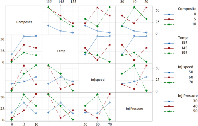
Interaction plot for tensile strength.
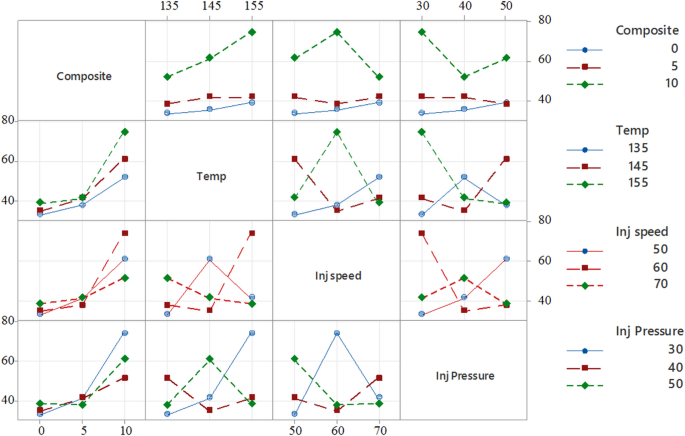
Figure 10 presents the interaction plots, illustrating how factors such as composition, temperature, injection speed, and injection pressure interactively influence the tensile strength of PLA/CCB composites. For example, in the plot comparing temperature and composition, the tensile strength increases from approximately 10 to over 50 MPa at 135 °C as the filler content rises from 0% to 10%. However, this trend reverses at higher temperatures; at 155 °C, increasing the composite content causes the tensile strength to drop from around 45 MPa to below 20 MPa, highlighting a significant interaction between these two parameters. Similarly, the subplot of injection speed versus injection pressure shows that tensile strength peaks at an injection speed of 60 mm/s and a pressure of 40 bar, while deviating from this combination results in a sharp decline, indicating the presence of non-linear interactions. The presence of non-parallel lines in most plots further confirms that the effect of one factor is heavily dependent on the level of another. These findings underscore the importance of considering parameter interactions collectively when optimizing processing conditions, rather than evaluating factors in isolation.
Young’s modulus
The ANOVA results summarized in Table 11 indicate that the injection molding process parameters have a statistically significant effect on the Young’s modulus of PLA/CCB composites, as evidenced by a P-value of 0.000 (P < 0.001). This confirms a highly significant influence of both the process parameters and composition on the stiffness of the composites. Among these factors, temperature and composition were identified as the most influential, contributing 38.58% and 20.14%, respectively. Injection speed and injection pressure also had notable effects, with contributions of 19.17% and 18.41%, respectively. Only 3.72% of the variation was attributed to experimental error, indicating excellent process control and repeatability. In addition, the regression model demonstrated a strong relationship between Young’s modulus and the process parameters. The model showed a high degree of accuracy and reliability, with a coefficient of determination (R2) of 97.95% and an adjusted R2 of 97.24%, confirming that the selected process parameters provided a good predictive fit for estimating the Young’s modulus of PLA/CCB composites.
Regression Eq.
$$begin{gathered} {text{YM}},=,{text{1121}}.{text{8}}, – ,{text{187}}.0{{text{F}}_{text{1}}} – {text{349}}.0{{text{F}}_{text{2}}},+,{text{536}}.0{{text{F}}_{text{3}}},+,{text{678}}.{text{4}}{{text{T}}_{text{1}}} hfill \ – {text{56}}.0{{text{T}}_{text{2}}}, – ,{text{622}}.{text{4}}{{text{T}}_{text{3}}}, – ,{text{19}}.{text{6}}{{text{S}}_{text{1}}} – {text{449}}.{text{6}}{{text{S}}_{text{2}}}, hfill \ +,{text{469}}.{text{2}}{{text{S}}_{text{3}}} – {text{477}}.{text{8}}{{text{P}}_{text{1}}}+{text{417}}.{text{1}}{{text{P}}_{text{2}}}+{text{6}}0.{text{7}}{{text{P}}_{text{3}}} hfill \ end{gathered}$$
(23)
Here, F1, F2, F3: Composite levels (0%, 5%, 10%), T1, T2, T3: Temperature levels (135 °C, 145 °C, 155 °C), S1, S2, S3: Injection speed levels (50, 60, 70 mm/s), P1, P2, P3: Injection pressure levels (30, 40, 50 bar), and YM: Young’s modulus (MPa).
Figure 11 compares the experimentally obtained Young’s modulus values with those predicted by the ANOVA-based regression Eq. (23). The percentage errors between the predicted and actual values were calculated to assess the model’s accuracy. Overall, most deviations fell within an acceptable range, confirming the strong predictive capability of the regression model. For instance, predicted values around 1115.79 MPa exhibited percentage errors between ± 3.88% and ± 14.09%, while predictions near 846.26 MPa showed errors ranging from ± 3.04% to ± 8.14%. Similarly, for values around 1062.41 MPa and 708.21 MPa, the deviations remained within ± 10%. Even at higher modulus values such as 3222.63 MPa, the model maintained reasonable accuracy, with errors ranging from ± 7.18% to ± 17.71%. Notably, for the lowest predicted modulus value of 107.97 MPa, the percentage error was as low as ± 0.03%. These findings confirm the reliability and robustness of the ANOVA-based regression model in accurately estimating Young’s modulus across a broad range of processing conditions for PLA/CCB composites.
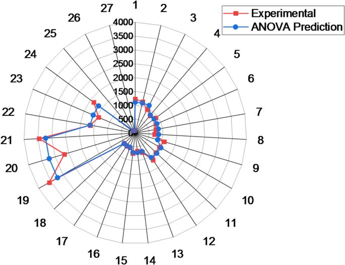
Young’s modulus prediction accuracy based on ANOVA model.
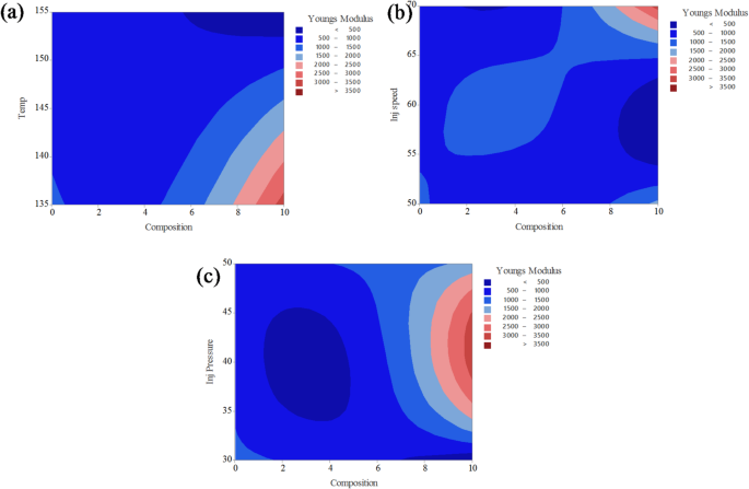
Contour plot analysis for Young’s modulus on (a) composition and temperature; (b) composition and injection speed; (c) composition and injection pressure.
The contour plots in Fig. 12 illustrate the combined effects of two process parameters on the Young’s modulus of PLA composites reinforced with CCB, while keeping the other parameters constant. In Fig. 12a, the interaction between composition and temperature shows that Young’s modulus significantly improves at higher filler contents, particularly above 7%, and at lower processing temperatures between 135 °C and 140 °C, where modulus values exceed 3000 MPa (represented by the red zone). In contrast, most of the plot remains dark blue, indicating modulus values below 1500 MPa, especially at lower compositions and higher temperatures. Figure 12b displays the combined effect of composition and injection speed, where moderately high modulus values (ranging from 2000 to 3000 MPa, shown in light red to red shades) are observed at higher compositions (8–10%) and injection speeds around 65 mm/s. However, a large portion of the plot remains blue, representing modulus values below 2000 MPa. In Fig. 12c, the interaction between composition and injection pressure reveals that Young’s modulus exceeds 3000 MPa when the composition is above 8% and the injection pressure is maintained between 40 and 45 bar. Similar to the other plots, the majority of this contour remains in the lower blue regions, indicating values under 2000 MPa. The color gradient, ranging from dark blue (< 500 MPa) to dark red (> 3500 MPa), effectively highlights the positive influence of increased CCB content and optimized processing parameters on enhancing the stiffness of PLA/CCB composites.
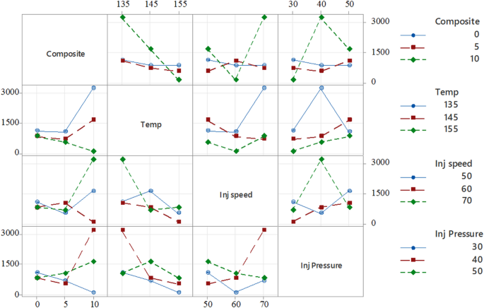
Interaction plot for Young’s modulus.
Figure 13 presents the interaction plots, demonstrating how factors such as composition, temperature, injection speed, and injection pressure collectively influence the Young’s modulus of PLA/CCB composites. For instance, in the plot comparing temperature and composition, the Young’s modulus increases sharply from approximately 1200 MPa to over 3000 MPa at 135 °C as the filler content rises from 0% to 10%. However, this trend reverses at 155 °C, where increasing the composite content results in a sharp decline in modulus, dropping from around 1200 MPa to nearly zero, which clearly indicating a strong interaction between these two parameters. Similarly, in the injection speed versus injection pressure subplot, the Young’s modulus reaches its peak at an injection speed of 60 mm/s and a pressure of 40 bar but decreases considerably at other parameter combinations, highlighting the presence of non-linear interactions. The appearance of non-parallel and intersecting lines across multiple plots further confirms that the effect of one process factor is highly dependent on the levels of the others. These findings emphasize the necessity of considering the combined interactions among processing parameters when optimizing for maximum stiffness, rather than evaluating each factor in isolation.
Hardness
The ANOVA results presented in Table 12 indicate that the injection molding process parameters have a statistically significant effect on the hardness of PLA/CCB composites, as confirmed by a P-value of 0.000 (P < 0.001). This highlights a strong influence of both the selected processing parameters and composition on the hardness performance of the composites. Among these factors, composition emerged as the most dominant, contributing 78.23% to the total variation, followed by temperature with a contribution of 10.87%. Injection speed and injection pressure also had measurable, though comparatively smaller, effects, contributing 2.81% and 4.55%, respectively. The remaining 3.55% was attributed to experimental error, indicating good process stability and repeatability. In addition, the regression analysis demonstrated a strong correlation between hardness and the processing parameters. The regression model, represented by Eq. (24), confirmed its robustness, achieving a coefficient of determination (R2) of 96.45% and an adjusted R2 of 94.87%. These values indicate high predictive accuracy and reliability in estimating the hardness of PLA/CCB composites under various processing conditions.
Regression Equation
$$begin{gathered} {text{Hardness }}left( {text{H}} right)={text{46}}.0{text{52}}, – ,{text{1}}0.{text{485}}{{text{F}}_{text{1}}}, – ,{text{5}}.{text{819}}{{text{F}}_{text{2}}},+,{text{16}}.{text{3}}0{text{4}}{{text{F}}_{text{3}}}, – ,{text{5}}.{text{185}}{{text{T}}_{text{1}}}, – ,0.{text{285}}{{text{T}}_{text{2}}}, hfill \ +,{text{5}}.{text{47}}0{{text{T}}_{text{3}}}, – ,0.{text{9}}0{text{7}}{{text{S}}_{text{1}}},+,{text{3}}.0{text{48}}{{text{S}}_{text{2}}}, – ,{text{2}}.{text{141}}{{text{S}}_{text{3}}},+,{text{3}}.{text{559}}{{text{P}}_{text{1}}}, – ,{text{3}}.{text{33}}0{{text{P}}_{text{2}}}, – ,0.{text{23}}0{{text{P}}_{text{3}}}. hfill \ end{gathered}$$
(24)
Here, F1, F2, F3: Composite levels (0%, 5%, 10%), T1, T2, T3: Temperature levels (135 °C, 145 °C, 155 °C), S1, S2, S3: Injection speed levels (50, 60, 70 mm/s), P1, P2, P3: Injection pressure levels (30, 40, 50 bar), and H: Hardness (HV).
Figure 14 presents a comparison between the experimentally measured and ANOVA-predicted hardness values for the PLA/CCB composites. The experimental hardness values ranged from 32.3 to 77, while the predicted values varied between 33.03 and 74.43. The percentage deviations between experimental and predicted results were generally below 10%, indicating strong agreement and high predictive accuracy of the regression model. For instance, an experimental hardness of 34 exhibited a deviation of approximately 2.96% from the predicted value of 33.03, while hardness values around 35.9 showed deviations close to 2.57%. Although a few data points displayed slightly higher deviations—such as an experimental value of 46.8 compared to a predicted 41.47—the majority of values remained well within acceptable limits. These findings confirm that the ANOVA-based regression model effectively captures the influence of processing parameters on the hardness of PLA/CCB composites and provides reliable predictions. This demonstrates the model’s practical value for process optimization, property prediction, and quality control in composite manufacturing.
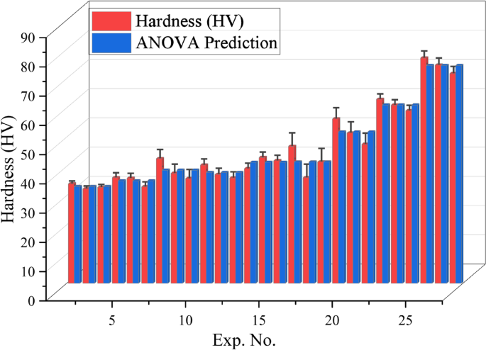
Hardness prediction accuracy based on ANOVA model.
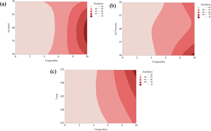
Contour plot analysis for hardness on (a) composition and injection speed; (b) Composition and injection pressure; (c) composition and temperature.
The contour plots in Fig. 15a–c illustrate the combined effects of two process parameters on the hardness of PLA composites reinforced with CCB, while keeping the other parameters constant. In Fig. 15a, the interaction between composition and injection speed reveals that hardness steadily increases as the CCB content exceeds 6%, reaching maximum values above 70 HV (indicated by dark red regions) at around 9–10% composition, largely independent of injection speed. Most of the lower composition region remains in light pink shades, representing hardness values below 50 HV. Figure 15b shows the combined effect of composition and injection pressure, where hardness values greater than 70 HV are achieved when the composition exceeds 8% and the injection pressure is maintained between 40 and 50 bar. In contrast, areas with composition below 6% consistently record hardness values under 50 HV. Similarly, Fig. 15c illustrates the interaction between composition and temperature, indicating that hardness exceeds 70 HV when the CCB content is above 8% and the processing temperature ranges between 140 °C and 150 °C. The color gradient, shifting from light pink (< 40 HV) to dark red (> 70 HV), consistently demonstrates that increasing CCB content has a pronounced positive effect on hardness across all processing conditions. Additionally, optimized ranges of injection speed, pressure, and temperature further enhance the material’s hardness performance, reinforcing the role of composition as the most dominant influencing factor.
Interaction plot for hardness.
Figure 16 presents the interaction plots, illustrating how composition, temperature, injection speed, and injection pressure collectively influence the hardness of PLA/CCB composites. In the plot comparing temperature and composition, hardness increases consistently with both parameters. At 155 °C, raising the composite content from 0% to 10% results in a sharp rise in hardness from approximately 40 HV to nearly 80 HV, indicating a strong synergistic interaction between these two factors. In contrast, the plot for injection speed versus injection pressure displays a more complex relationship. Peak hardness is achieved at an injection speed of 60 mm/s and an injection pressure of 40 MPa, while other combinations produce more varied and less predictable responses. The presence of intersecting and non-parallel lines across the interaction plots confirms that the effect of one process parameter is highly dependent on the levels of the others. These trends emphasize that maximizing the hardness of PLA/CCB composites requires a simultaneous and balanced optimization of all processing parameters, rather than adjusting them in isolation.
Machine learning
Tensile strength
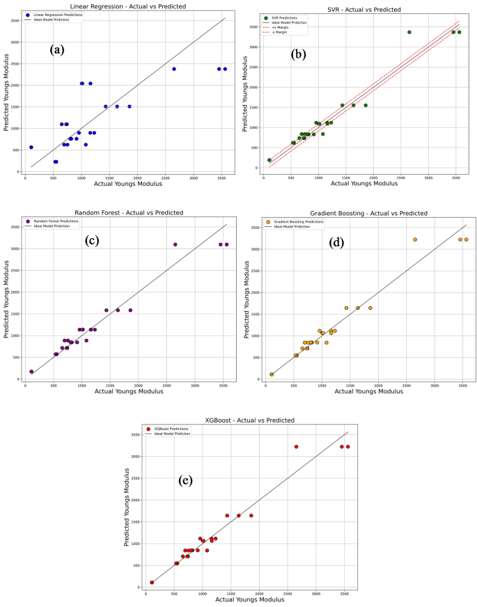
Figure 17a–e compares the experimentally measured tensile strength values of PLA/CCB composites with predictions from various machine learning models, including Linear Regression, Support Vector Regression (SVR), Random Forest Regression, Gradient Boosting, and Extreme Gradient Boosting (XG-Boost). In each plot, colored dots represent the model’s predicted values, while a 45° reference line indicates perfect prediction accuracy. In Fig. 17a, the Linear Regression model, represented by blue dots, shows considerable deviations from the ideal line, reflecting its limited ability to capture the non-linear relationships within the data. This is further supported by its low R2 value of 0.7965 and high error metrics: MSE of 76.53, RMSE of 8.75, MAE of 7.79, and MAPE of 69.87%. Figure 17b depicts the performance of the SVR model, shown with green dots. Here, predictions align more closely with the diagonal line, although some dispersion remains at the data extremes. The model delivers a significantly improved R2 of 0.9829, with reduced errors: MSE of 6.45, RMSE of 2.54, MAE of 1.98, and MAPE of 18.68%. In Fig. 17c, the Random Forest model, represented by purple dots, displays even tighter clustering along the reference line, indicating further enhancement in prediction accuracy. It achieves an R2 of 0.9857, MSE of 5.38, RMSE of 2.32, MAE of 1.64, and MAPE of 13.92%. Figure 17d presents the Gradient Boosting model, shown with orange dots, where predictions are closely aligned with the ideal line, reflecting excellent accuracy and generalization. This model records an R2 of 0.9878, MSE of 4.60, RMSE of 2.15, MAE of 1.19, and MAPE of 6.67%. Figure 17e illustrates the XG-Boost model’s performance, with red dots almost perfectly aligned along the 45° line. It matches the performance of Gradient Boosting with an R2 of 0.9878, MSE of 4.60, RMSE of 2.15, MAE of 1.19, and MAPE of 6.67%, confirming its exceptional predictive capability. Overall, these results highlight that ensemble-based models, particularly Gradient Boosting and XG-Boost deliver superior prediction accuracy and reliability for estimating tensile strength, outperforming simpler models like Linear Regression and SVR.
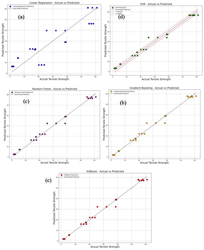
Comparison of actual vs. predicted tensile strength using machine learning models (a) linear regression; (b) support vector regression (SVR); (c) random forest; (d) gradient boosting; (e) XG-boost.
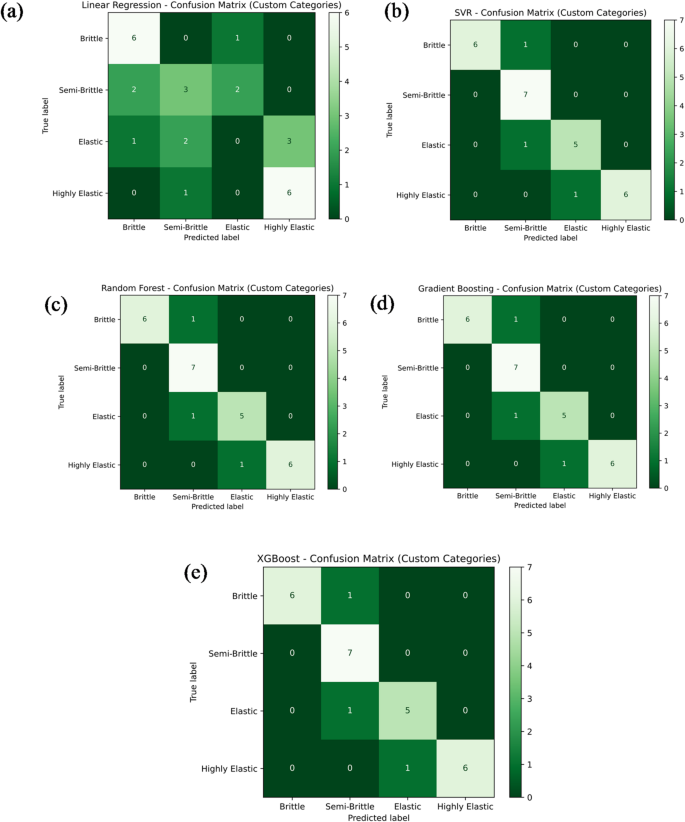
Figure 18a–e presents the classification performance of various machine learning models — namely Linear Regression, Support Vector Regression (SVR), Random Forest Regression, Gradient Boosting, and XG-Boost — in predicting the tensile strength category of PLA/CCB composites based on their material behavior: brittle, semi-brittle, elastic, and highly elastic. In Fig. 18a, the Linear Regression model achieves a classification accuracy of 60.7%, correctly identifying 6 brittle, 3 semi-brittle, 2 elastic, and 6 highly elastic samples. However, several misclassifications are observed, including 1 brittle sample incorrectly classified as elastic, 2 semi-brittle samples misclassified as brittle and elastic, 1 elastic sample classified as brittle, 3 elastic samples as highly elastic, and 1 elastic sample again as highly elastic. In comparison, Fig. 18b–e display the classification results of SVR, Random Forest, Gradient Boosting, and XG-Boost models. Each of these models achieved a notably higher classification accuracy of 85.7%, correctly categorizing 6 brittle, 7 semi-brittle, 5 elastic, and 6 highly elastic samples. The few misclassifications observed included 1 semi-brittle sample classified as brittle, another semi-brittle as elastic, and 1 elastic sample classified as highly elastic. Overall, these figures collectively provide a clear comparison of the classification accuracy and predictive reliability of the tested models. Ensemble learning techniques like Random Forest, Gradient Boosting, and XG-Boost outperformed Linear Regression and SVR, consistently delivering higher classification accuracy across different material behavior categories.
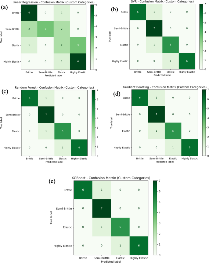
Confusion matrix for machine learning model predicting tensile strength by (a) linear regression; (b) support vector regression (SVR); (c) random forest; (d) gradient boosting; (e) XG-Boost.
Young’s modulus
Figure 19a–e compares the experimentally measured values of Young’s modulus with the predictions obtained from various machine learning models, namely Linear Regression, Support Vector Regression (SVR), Random Forest Regression, Gradient Boosting, and Extreme Gradient Boosting (XG-Boost). In each plot, the predicted values are represented by colored dots plotted against a 45° reference line, which signifies perfect prediction accuracy. As shown in Fig. 19a, the Linear Regression model (blue dots) exhibits noticeable deviations from the reference line, indicating its inability to effectively capture the inherent non-linear relationships present in the dataset. This limitation is evident from its relatively poor performance indicators: an R2 of 0.622, MSE of 277,846.6, RMSE of 527.11, MAE of 410.78, and MAPE of 79.60%. In comparison, the SVR model illustrated in Fig. 19b with green dots shows improved alignment with the diagonal, although some dispersion remains. It achieves a notably higher R2 value of 0.9562, along with considerably lower error metrics: MSE of 32,194.02, RMSE of 179.43, MAE of 118.87, and MAPE of 17.50%. Further improvement is observed with the Random Forest model in Fig. 19c (purple dots), where the predicted values cluster more tightly around the 45° line. This enhanced performance is reflected by an R2 of 0.9579, MSE of 30,921.54, RMSE of 175.85, MAE of 123.73, and MAPE of 15.15%. The Gradient Boosting model, shown in Fig. 19d with orange dots, demonstrates even stronger predictive accuracy, with predictions closely following the ideal line. This model records an R2 of 0.9628, MSE of 27,313.71, RMSE of 165.27, MAE of 105.25, and MAPE of 7.72%, indicating excellent generalization and minimal prediction errors. A comparable level of performance is achieved by the XG-Boost model, depicted in Fig. 19e with red dots. Its predicted values almost perfectly overlap the 45° line, and it records identical performance metrics to those of Gradient Boosting. Overall, the results clearly indicate that tree-based ensemble models—particularly Gradient Boosting and XG-Boost—are highly effective in capturing complex non-linear patterns within the data. This is critically important for reliably predicting the mechanical behavior of materials, which can be adversely affected by factors such as thermal degradation and molecular reorientation during the cooling phase. Accurate modeling of these effects is therefore essential to ensure optimal material performance and structural integrity.
Comparison of actual vs. predicted young’s modulus using machine learning models: (a) linear regression; (b) support vector regression (SVR); (c) random forest; (d) gradient boosting; (e) XG-Boost.
Figure 20a–e presents the classification performance of various machine learning models in predicting Young’s modulus categories for different material types, including brittle, semi-brittle, elastic, and highly elastic. The models evaluated include Linear Regression, Support Vector Regression (SVR), Random Forest Regression, Gradient Boosting, and Extreme Gradient Boosting (XG-Boost). As shown in Fig. 20a, the Linear Regression model correctly classified 6 as brittle, 3 as semi-brittle, and 6 as highly elastic samples, while failing to identify any elastic samples. This resulted in an overall classification accuracy of 53.6%. The remaining samples were misclassified as follows: 1 as a brittle sample incorrectly labelled as elastic; 2 as semi-brittle samples misclassified as brittle and elastic, respectively; 1 as an elastic sample labelled as brittle; 2 as elastic samples as semi-brittle; 3 as elastic samples as highly elastic; and 1 as an additional elastic sample also misclassified as highly elastic. In contrast, the other four models—SVR, Random Forest Regression, Gradient Boosting, and XG-Boost—demonstrated significantly higher classification accuracies, each achieving 85.7%, as depicted in Fig. 20b–e. These models successfully identified 6 as brittle, 7 as semi-brittle, 5 as elastic, and 6 as highly elastic samples correctly. A few misclassifications were noted: one semi-brittle sample was wrongly classified as brittle, another as elastic, and one elastic sample was incorrectly labelled as highly elastic. In summary, these classification results highlight the superior predictive capability of tree-based ensemble models and SVR over Linear Regression for categorizing material behavior based on Young’s modulus. Accurate classification is essential for evaluating the structural response of materials under mechanical loads, particularly considering variations in material composition and processing conditions.
Confusion matrix for the machine learning model predicting Young’s modulus via (a) linear regression; (b) support vector regression (SVR); (c) random forest; (d) gradient boosting; e) XG-Boost.
Hardness
Figure 21a–e compares the predictions of several machine learning models with the experimentally measured hardness values. The models evaluated include Linear Regression, Support Vector Regression (SVR), Random Forest Regression, Gradient Boosting, and Extreme Gradient Boosting (XG-Boost). In each plot, the predicted values are represented by colored dots plotted against a diagonal reference line, which represents perfect prediction accuracy. As shown in Fig. 21a, the Linear Regression model (blue dots) displays considerable deviation from the reference line, reflecting its limited ability to model the non-linear relationships inherent in the dataset. This limitation is evident from its moderate performance metrics, with an R2 of 0.8088, MSE of 33.35, RMSE of 5.775, MAE of 4.5956, and MAPE of 10.3%. The SVR model, illustrated in Fig. 21b with green dots, shows a marked improvement, with predictions more closely aligned to the reference line, though some dispersion persists. It achieves a higher R2 of 0.9598, with substantially reduced error values: MSE of 7.004, RMSE of 2.6466, MAE of 2.1462, and MAPE of 4.87%. Further enhancement is observed in the Random Forest model, shown in Fig. 21c with purple dots, where the predicted values cluster more tightly around the diagonal. This model records an R2 of 0.9638, MSE of 6.3173, RMSE of 2.5134, MAE of 1.9873, and MAPE of 4.4988%, indicating strong predictive accuracy. The Gradient Boosting model, represented by orange dots in Fig. 21d, delivers even better performance, with predictions closely following the reference line. It achieves an R2 of 0.9645, MSE of 6.1958, RMSE of 2.4891, MAE of 1.9383, and MAPE of 4.4061%, confirming excellent prediction consistency and generalization capability. Similarly, the XG-Boost model, shown by red dots in Fig. 21e, achieves nearly identical performance to Gradient Boosting, with its predictions almost perfectly overlapping the reference line. Its comparable R2 and error metrics further affirm its accuracy. Overall, these results clearly demonstrate that tree-based ensemble models—particularly Gradient Boosting and XG-Boost—offer superior predictive performance, effectively capturing the complex non-linear patterns in the hardness data. This underlines their suitability for reliably forecasting mechanical properties in materials research.
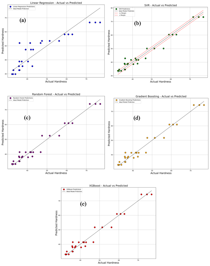
Comparison of actual vs. predicted hardness using machine learning models: (a) linear regression; (b) support vector regression (SVR); (c) random forest; (d) gradient boosting; (e) XG-Boost.
Figure 22a–e presents the classification performance of various machine learning models in categorizing material hardness into four categories: brittle, semi-brittle, elastic, and highly elastic. The models assessed include Linear Regression, Support Vector Regression (SVR), Random Forest Regression, Gradient Boosting, and Extreme Gradient Boosting (XG-Boost). As illustrated in Fig. 22a, the Linear Regression model achieved a classification accuracy of 53.6%, correctly identifying 6 as brittle, 2 as semi-brittle, 5 as elastic, and 6 as highly elastic samples. The model’s misclassifications comprised 1 as brittle sample incorrectly labelled as semi-brittle; 2 as semi-brittle samples as brittle; 3 as semi-brittle samples as elastic; 1 as elastic sample as brittle; and 1 as highly elastic sample misclassified as elastic. In comparison, the SVR model shown in Fig. 22b demonstrated improved performance, attaining an accuracy of 85.7%. It accurately classified 5 as brittle, 3 as semi-brittle, 5 as elastic, and 6 as highly elastic samples. The remaining misclassifications included 2 as brittle samples as semi-brittle; 1 as semi-brittle sample as brittle; 3 as semi-brittle samples as elastic; 1 as elastic sample as semi-brittle; and 1 as highly elastic sample as elastic. The Random Forest Regression, Gradient Boosting, and XG-Boost models, presented in Fig. 22c–e, each achieved a classification accuracy of 67.87%. These models correctly identified 5 as brittle, 6 as semi-brittle, 2 as elastic, and 6 as highly elastic samples. However, their misclassifications involved 2 as brittle samples as semi-brittle, 1 as semi-brittle sample as brittle, 4 as elastic samples misclassified as semi-brittle, and 1 as highly elastic sample as elastic. In summary, these figures highlight the comparative classification performance of the different machine learning models in predicting material hardness categories. Notably, the SVR model outperformed the others in terms of classification accuracy, while the tree-based ensemble models exhibited moderate yet consistent predictive capability, effectively capturing the trends in material hardness behavior across the defined categories.
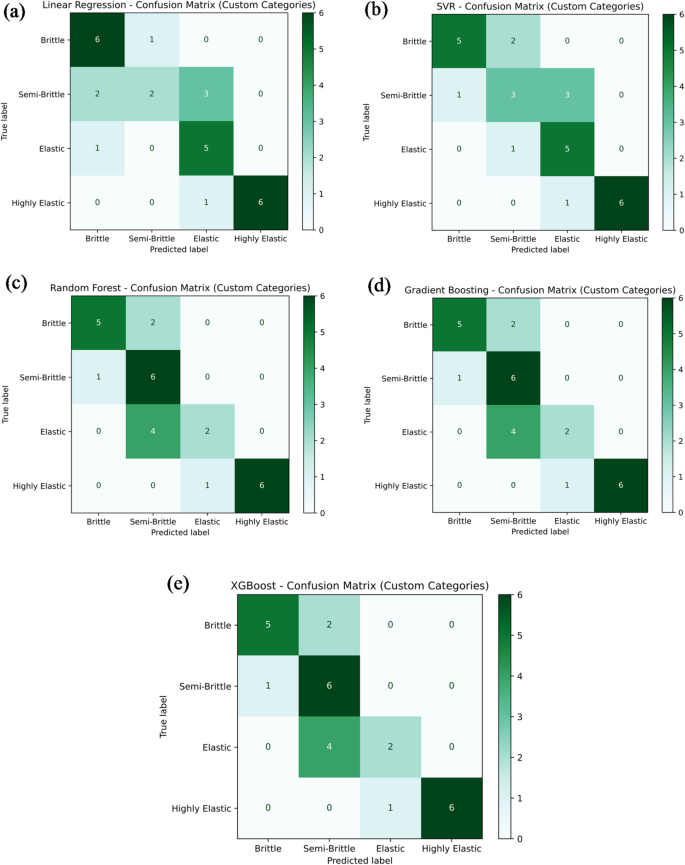
Confusion matrix for machine learning model predicting hardness by (a) linear regression; (b) support vector regression (SVR); (c) random forest; (d) gradient boosting; (e) XG-Boost.
Figure 23 illustrates the influence of injection molding processing parameters on the mechanical properties—Tensile Strength, Young’s Modulus, and Hardness—through the analysis of Pearson correlation coefficients. The heatmap reveals a strong negative correlation between Composition and Hardness (− 0.83) and a moderate negative correlation with Tensile Strength (− 0.57). This suggests that increasing the proportion of certain compositional elements, such as fillers or additives, tends to produce softer materials with diminished tensile strength. Similarly, Temperature exhibits a notable negative correlation with both Tensile Strength (− 0.65) and Young’s Modulus (− 0.62), indicating that higher processing temperatures can adversely affect the mechanical performance of the material. This reduction in strength and stiffness may be attributed to thermal degradation or alterations in molecular alignment during the cooling phase. In contrast, a moderate positive correlation (0.58) is observed between Tensile Strength and Young’s Modulus, which is consistent with typical mechanical behavior where materials with higher tensile strength generally exhibit greater stiffness. Interestingly, both Injection Speed and Injection Pressure show only weak correlations with the mechanical properties, implying that their effects are either less significant or potentially nonlinear when compared to the dominant influences of Composition and Temperature. Overall, this analysis underscores the importance of carefully optimizing both the material composition and processing temperature to achieve desirable mechanical performance in injection-molded components.
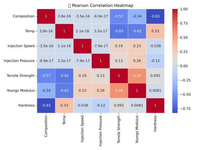
Correlation map between process parameters and mechanical property.
Cross-validation of ML
To evaluate the robustness and generalization capability of the machine learning models, a k-fold cross-validation (CV) approach was adopted, where the dataset was divided into five subsets and each was used once as a test set while the remaining four served for training. The comparison between CV and train–test R2 values showed strong consistency with limited deviation. For tensile strength, SVR, Gradient Boosting, and XGBoost attained CV R2 values of 0.936–0.941, compared to train–test values near 0.988, resulting in an error margin of ~ 4.7–5.2%. Hardness predictions yielded CV R2 values of 0.879–0.885, closely matching train–test values of 0.954–0.965, with an error of ~ 0.07–0.09. Young’s modulus displayed slightly higher variation, with CV R2 of 0.791–0.827 against train–test values of 0.956–0.963, producing an error of ~ 0.13–0.14. Overall, Gradient Boosting and XGBoost provided the best performance, confirming reliable prediction approximately 5% for tensile strength, under 10% for hardness, and 13% for Young’s modulus, confirming their robustness for modelling PLA/CCB composites.
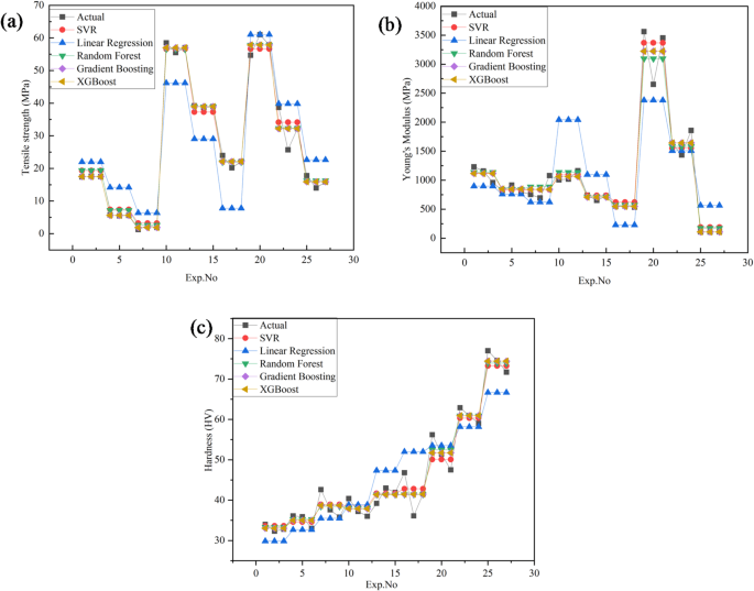
Comparison of experimental results with ML models (a) tensile strength; (b) Young’s modulus; (c) hardness.
Figure 24a compares the experimentally measured and predicted values of tensile strength across 27 experimental runs (Exp. No. 1–27). Predictions were generated using Linear Regression, Support Vector Regression (SVR), Random Forest, Gradient Boosting, and Extreme Gradient Boosting (XG-Boost). Among these, Gradient Boosting and XG-Boost provided the closest match to the experimental data, particularly in Exp. No. 1–3, 10–12, and 22–24, where the predicted values nearly overlapped with the actual measurements. Figure 24b presents the results for Young’s modulus under the same modeling approaches. Similar to tensile strength, Gradient Boosting and XG-Boost achieved the highest accuracy, showing strong alignment with the experimental results in Exp. No. 1–3, 10–12, and 22–24. These models demonstrated minimal deviation, underscoring their capability to capture the underlying mechanical behavior with high reliability.
Figure 24c illustrates the comparison for hardness. While all models produced reasonable predictions, Gradient Boosting and XG-Boost again outperformed the others, especially in Exp. No. 18–27, where near-perfect agreement between predicted and measured values was observed. This consistent performance highlights the robustness of these models in capturing complex nonlinear patterns across different mechanical properties.