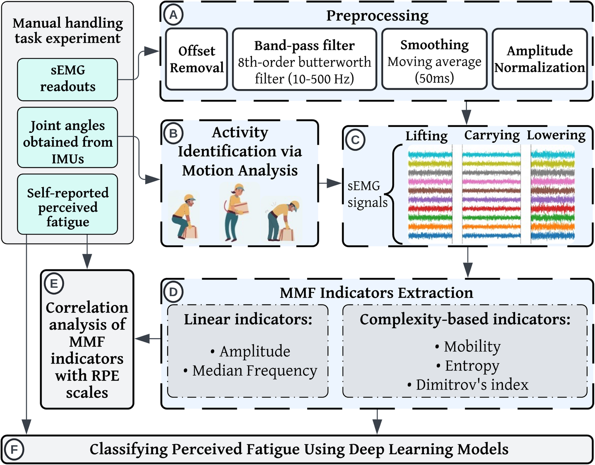
The flowchart of the procedure in this study includes: A Preprocessing the sEMG signals; B Manual handling task segmentation using the joint angles obtained by IMUs; C Segmenting sEMG signals based on IMU-derived time windows; D Identifying and extracting linear and complexity-based MMF indicators; E Analyzing the correlation between MMF indicators and RPE scales; and F Classifying performance fatigue via a long short-term memory (LSTM) model and a convolutional neural network combined with LSTM (CNN-LSTM) using MMF indicators
Figure 1 provides an overview of the experimental process followed in this study, with subsequent sections offering detailed explanations of each step .
Experimental procedure
The study recruited eight able-bodied male participants (average age: 24 ± 2 years, average body mass: 73 ± 11 kg, average body height: 179 ± 4 cm). The participants were instructed to perform repetitive cycles of a manual handling task including lifting a 16-lbs load from a 15-cm high table, turning, placing it on a 75-cm high table, and going to the rest position; lifting the load again from the 75-cm high table, turning, and placing it back on the 15-cm high table (Fig. 2). The participant performed these movements repeatedly and reported their perceived fatigue level using the Borg RPE scale every 2 min. The experiment concluded when participants reported a fatigue level of 9 out of 10 on the RPE scale. Participants performed an average of 146 ± 43 cycles, and each participant completed two recording sessions on different days, each starting in a rested state to minimize potential carryover effects such as residual fatigue or motor adaptation. The Research Ethics Board of the University of Alberta approved the experimental protocol (Approval no. Pro00089234), and the participants provided written consent prior to testing. We used the data used in our previous publications [4, 8].
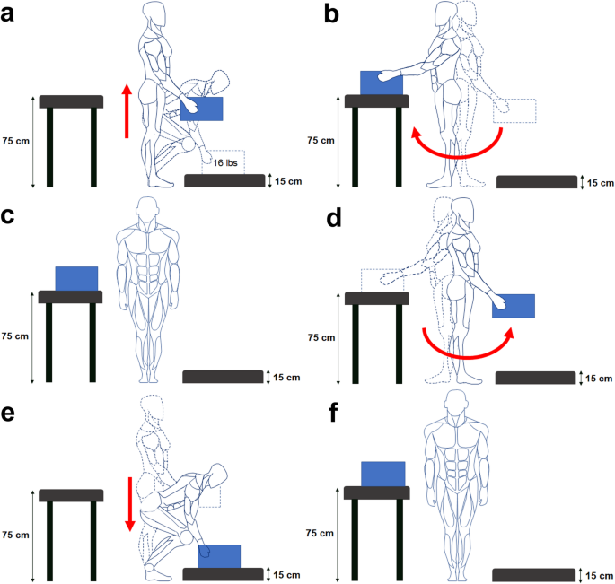
Manual handling task cycle including lifting (a), carrying, (b–d), and lowering (e) activities, followed by a resting position (f)
Ten sEMG sensors (Trigno, Delsys, USA) were placed on the following muscles on the right side of the participants’ bodies, as all participants were right-handed: Biceps Brachii (Biceps), Flexor Carpi Radialis, Trapezius, Deltoideus Posterior, Erector Spinae Longissimus (L), Erector Spinae Iliocostalis (I), Rectus Femoris, Tibialis Anterior, Biceps Femoris, and Lateral Gastrocnemius with a sampling frequency of 1200 Hz. The sEMG data were first mean-subtracted and then filtered using a zero-lag, 8th-order Butterworth bandpass filter set to 10–500 Hz. Following this, the data were smoothed with a 50 ms window size. The sEMG time series was then normalized to the maximum amplitude during the first five cycles (non-fatigue states) of the experiment to help reduce inter-session variability.
Additionally, seven IMUs (MTws, Xsens Technologies, NL) were positioned on their sternum, sacrum, right upper arm, forearm, thigh, shank, and foot to monitor joint angles’ kinematics, with a sampling frequency of 100 Hz. Similar to the EMG setup, IMUs were placed only on the right side, as all participants were right-handed. This setup helped reduce the number of sensors required, minimizing participant discomfort and motion constraints during the prolonged trials. Prior to the main experiment, a functional calibration was performed according to the protocol outlined in [23]. This calibration aimed to synchronize the inertial frames of the IMUs with the body’s anatomical frames for measuring joint angles. Participants were instructed to maintain stillness for 5 s, followed by performing ten flexions and extensions of both legs and arms with locked knee and elbow joints. Subsequently, the IMU readings were utilized to calculate body joint angles based on the orientation derived from the Xsens sensor fusion algorithm. Data was preprocessed using MATLAB R2022a (The MathWorks Inc., Natick, MA, USA).
Data segmentation based on activities
Our experiment involved a manual handling task with different activities of lifting, carrying, and lowering, and each of them included different body movements and muscle engagements; therefore, the sEMG recordings were first segmented based on these three distinct activities. This segmentation was performed using joint angle data processed in OpenSim, which simulated the motion and identified activity boundaries according to predefined activity definitions. Additionally, each muscle primarily influences the motion of one or more joints and the positions of adjacent joints can also affect the level of muscle engagement due to changes in torque demands, moment arms, and muscle–tendon length. Specifically: (1) Biceps and Flexor Carpi Radialis were associated with the elbow & shoulder flexion/extension, (2) Trapezius and Deltoideus Posterior influenced the shoulder flexion/extension, (3) Erector Spinae L and I influenced the trunk flexion/extension, (4) Rectus Femoris and Biceps Femoris influenced the hip and knee flexion/extension, (5) Tibialis Anterior and Lateral Gastrocnemius influenced the ankle and knee flexion/extension. The sEMG signals were further segmented based on the relevant joints’ ROM, dividing each into two equal segments (0–50% and 50–100% of the ROM).
sEMG data processing
Amplitude analysis
Root Mean Square (RMS) values were used to characterize sEMG signal amplitude for monitoring muscle fatigue [24]. For a discrete signal with N samples, the RMS can be computed using the following formula:
$$:RMS=:sqrt{frac{1}{N}{int:}_{i=1}^{N}x{left[iright]}^{2}}$$
(1)
Where (:xleft[iright]) represents each sample within the analyzed sEMG signal segment.
As muscle fatigue progresses, the sEMG amplitude generally rises due to the recruitment of additional motor units, and potentially, their excitation at higher firing frequencies to compensate for the declining force-generating capacity of individual muscle fibers. Consequently, higher RMS values are expected in the later stages of RPE scales.
Spectral analysis
This approach identifies muscle fatigue by observing a shift in the power spectrum of sEMG signals toward lower frequencies, as indicated by the median frequency. The median frequency is calculated using the following equation:
$$:{int:}_{0}^{MDF}PSDleft(fright)df=:{int:}_{MDF}^{infty:}PSDleft(fright)df=frac{1}{2}{int:}_{0}^{infty:}PSDleft(fright)df$$
(2)
Where (:PSDleft(fright)) is the power spectral density at a given frequency (:f), calculated by the spectrogram function, which performs the Short-Time Fourier Transform of the preprocessed signal [25]. This process involved segmenting the signal with a 128-sample window, 64-sample overlap, and 256 Fast Fourier Transform points, with a sampling frequency of 1200 Hz. The spectrogram function provided the PSD matrix, reflecting the power at various frequencies and times, which was used for further analysis.
Mobility
Mobility is quantified as the square root of the ratio of the variance of the signal’s first derivative to the variance of the original signal [22] calculated as follows:
$$:Mobility=:sqrt{frac{{{sigma:}_{1}}_{x1}^{x2}}{{{sigma:}_{0}}_{x1}^{x2}}}:$$
(3)
where (:{{sigma:}_{0}}_{x1}^{x2}) and (:{{sigma:}_{1}}_{x1}^{x2}) are the variance of the sEMG signal and the variance of the first derivative of the sEMG signal, respectively. Both were computed over the full duration of each activity segment (i.e., lifting, carrying, or lowering), with (:{x}_{1}) and (:{x}_{2}) denoting the start and end time points of each segment.
As fatigue sets in, the mobility of the sEMG signal is expected to decrease due to a reduction in conduction velocity [22].
Entropy
Fuzzy entropy, a measure of complexity and regularity in time-series data, was investigated in this study due to its demonstrated robustness in assessing MMF. Fuzzy entropy was computed using the following procedure [16]:
-
1.
The sEMG time-series were divided into overlapping intervals of length (:m).
-
2.
For two sEMG intervals (:{S}_{i}=[{x}_{1},{x}_{2},dots:,:{x}_{m}]) and (:{S}_{j}=[{y}_{1},{y}_{2},dots:,:{y}_{m}]), the distance was calculated as:
$$:{d}_{i,j}^{m}=text{m}text{a}text{x}left(right|{x}_{1}-{y}_{1}|,|{x}_{2}-{y}_{2}|,dots:,|{x}_{m}-{y}_{m}left|right)$$
(4)
-
3.
For each pair of intervals, the similarity function was calculated as:
$$:{Omega:}left({d}_{i,j}^{m},text{n},text{r}right)=text{e}text{x}text{p}(-frac{{left({d}_{ij}^{m}:right)}^{n}}{r})$$
(5)
Where (:r) is the similarity threshold and (:n) is the power of the similarity function.
-
4.
(:{C}_{i}^{m}left(rright)), the similarity for interval (:i), was calculated as the average similarity across all other intervals (:j) as:
$$:{C}_{i}^{m}left(rright)={left(N-m+1right)}^{-1}{sum:}_{j=1,jne:i}^{N-m+1}{Omega:}({d}_{i,j}^{m},text{r})$$
(6)
Where N is the total number of sEMG time-serious data points.
-
5.
(:{C}^{m}left(rright)) was calculated as the average of (:{C}_{i}^{m}left(rright)) for all the intervals.
-
6.
Previous steps were repeated for intervals of length (:m+1) to calculate (:{C}^{m+1}left(rright)).
-
7.
Finally, the fuzzy entropy was calculated as:
$$:FuzzyEnleft(m,n,r,Nright)=-text{l}text{n}left(frac{{C}^{m+1}left(rright)}{{C}^{m}left(rright)}right)$$
(7)
The fuzzy entropy was calculated using the FuzzyEn MATLAB function [26] with an embedding dimension of (:m=2), a power factor of (:n=2) for the similarity function, and a similarity threshold of (:r=0.25) [27]. In higher fatigue stages, lower entropy values are anticipated due to the decreased complexity of sEMG signals, which is caused by a reduction in the number of active motor units [16].
Dimitrov’s index
To address the low sensitivity of traditional spectral parameters like mean frequency and median frequency for muscle fatigue monitoring, previous studies investigated the relationship between the sEMG power content in low and high frequencies [28]. However, a challenge is defining the boundaries of the high- and low-frequency bands, as their selection can significantly impact the interpretation of muscle fatigue. To overcome this issue, the Dimitrov’s index, a highly sensitive spectral metric, has been proposed. It effectively defines these boundaries using frequency weighting factors, as shown in Eq. 8. The Dimitrov’s index is derived from sEMG spectral characteristics using FFT. Here, the Dimitrov’s index [28] is calculated in the band frequency from 10 Hz to 500 Hz:
$$:FI=frac{underset{f=10}{overset{500}{int:}}{f}^{-1}.PSleft(fright).df}{underset{f=10}{overset{500}{int:}}{f}^{5}.PSleft(fright).df}$$
(8)
Where (:f) denotes frequency (which is the variable of integration), (:PSleft(fright)) is the sEMG power-frequency spectrum as a function of frequency (:f). (:{f}^{-1}) is a frequency weighting factor that gives more emphasis to lower frequencies, increasing their contribution and highlighting the power in the lower frequency range of the sEMG signal. Conversely, (:{f}^{5}) in the denominator is a frequency weighting factor that prioritizes higher frequencies by assigning more weight to larger frequency values, thereby focusing on the power in the higher frequency range.
As fatigue progresses, the Dimitrov’s index is expected to increase due to the higher power spectral density in the low and ultra-low frequencies compared to the higher frequencies in the higher fatigue stages [28].
Statistical analysis
Our approach aimed to initially investigate the correlation between the RPE scales, known as a perceived fatigue evaluator, and the MMF indicator calculated in this study. Thus, Spearman’s correlation coefficients and their corresponding p-values were calculated between each of the MMF indicators and fatigue levels (RPE scales of 1 to 10), utilizing the Fisher’s Z transformation and the generalized Bonferroni-Holm procedure, respectively [29, 30]. Spearman’s correlation was chosen because the analysis focused on monotonic, rather than linear, relationships between the MMF indicators and fatigue levels. For each RPE level, 10 segments were randomly sampled for each activity type (lifting, carrying, and lowering) to reduce autocorrelation and maintain consistency across participants, and MMF indicators were calculated over the full duration of each segment without additional windowing.
Spearman’s correlation coefficients were computed separately for each session between each MMF indicator and RPE scale. For analysis, correlations from the two sessions of each participant were first averaged (after Fisher Z-transformation) to obtain a single value per participant. The resulting correlation coefficients were transformed using Fisher’s Z transformation and averaged to obtain a group-level correlation value, which was then back-transformed to obtain the final reported Spearman’s ρ. Corresponding session-level p-values were adjusted for multiple comparisons using the generalized Bonferroni-Holm procedure. All statistical analyses were conducted in MATLAB using built-in and custom-written functions.
Multi-class fatigue detection
Then, we developed deep learning algorithms to classify multiple stages of perceived fatigue using the MMF indicators as inputs. For this purpose, the extracted MMF indicators from 5 consecutive repetitions were grouped together into a window and labeled into five discrete fatigue level bins using the reported RPE scales: 1–2, 3–4, 5–6, 7–8, and 9–10. The five fatigue levels were chosen because they provided reasonable accuracy while enabling multi-level classification without overcomplicating the process. We first used a long short-term memory (LSTM) network to capture temporal dependencies and complex sequential patterns in time-series data [31]. The model was developed using TensorFlow, incorporating regularization techniques and the Adam optimizer to enhance training efficiency and prevent overfitting. The neural architecture consisted of three LSTM layers with progressively smaller units: 128, 64, and 32, respectively. Each LSTM layer utilized L2 regularization with a strength of 0.01 to mitigate overfitting, and dropout was applied with a rate of 0.5 following each LSTM layer to further address overfitting. The model concluded with three dense layers with 32, 16, and 8 neurons, respectively, each employing the Rectified Linear Unit (ReLU) activation function. The output layer was comprised of five neurons with a SoftMax activation function designed to produce class probabilities corresponding to the five bins of RPE ratings. Leave-one-out cross-validation (LOOCV) was performed to ensure the model’s generalizability across different subjects. This method involved training the model on data from all but one participant and evaluating it on the excluded participant, ensuring a solid assessment of the model’s performance across diverse data subsets.
To improve predictive accuracy by capturing spatial dependencies of MMF indicators, a CNN-LSTM architecture was implemented. The CNN part of the model included two convolutional layers with 64 and 32 filters, respectively, using a kernel size of 3 and ‘tanh’ activation. Max-pooling layers with a pool size of 2 followed each convolutional layer to reduce spatial dimensions. These convolutional layers were followed by LSTM layers to capture temporal dynamics, allowing the model to learn both spatial and temporal dependencies in the data.