This section provides a comprehensive examination of the methodologies employed in forecasting wind energy generation using the most effective machine learning models, such as Random Forest and XGBoost. The discussion encompasses data preprocessing, feature selection, model training, validation, and performance evaluation. Additionally, it addresses the modeling of various components of the WECS within MATLAB Simulink, including wind turbine dynamics, power electronics, and control strategies, to facilitate a thorough system analysis.
Machine learning framework
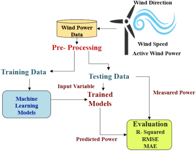
Figure 1 illustrates a framework for predicting wind power utilizing machine learning models. Initially, wind power data undergoes pre-processing and is subsequently divided into training and testing datasets. The Random Forest and XGBoost models are developed using the training data. These trained models are then employed to forecast power output by evaluating the input variables from the testing dataset. The performance of the models is assessed by comparing the predicted and actual power outputs, using metrics such as R-squared, Root Mean Square Error (RMSE), and Mean Absolute Error (MAE).
Workflow diagram for machine learning models.
The wind speed data from the MERRA-2 dataset constitutes the primary input feature for the ML models. An exploratory data analysis was performed to identify patterns and relationships within the data, and missing values were addressed to maintain data integrity. To enhance prediction accuracy, additional derived features, such as rolling averages and wind speed fluctuations, were engineered43. Preprocessing is a critical step in ensuring that raw wind power data is clean, consistent, and suitable for training machine learning models, involving several intricate processes. Missing values, which may arise from sensor failures, connectivity issues, or other data collection problems, were addressed using various techniques. This included mean or median imputation, which replaces missing values with the average or median of the corresponding variable, and interpolation methods such as linear or polynomial interpolation, which estimate missing values based on surrounding data patterns. Advanced machine learning models were also employed to predict missing values using features from other datasets. In instances where imputation was impractical, rows or attributes with a high percentage of missing data were removed.
Outlier detection and removal were performed to mitigate the impact of data points that significantly deviated from typical values, as such anomalies can distort model training. Techniques such as the Z-score method, interquartile range (IQR), and machine learning-based anomaly detection were employed. Since wind speed is measured in meters per second and often appears alongside variables with differing scales, normalization (scaling values between 0 and 1) or standardization (scaling to a mean of 0 and standard deviation of 1) was used to ensure that all features contributed equally during model training. Feature engineering was applied to enhance model performance by creating new variables that more accurately capture the underlying relationships in the data. For instance, wind direction and speed were combined to create vector representations, shifting medians and rolling averages were calculated to track temporal trends, and wind speeds were categorized into three classes: low, medium, and high. To ensure that only the most relevant variables were included, feature selection and dimensionality reduction techniques such as Principal Component Analysis (PCA), mutual information, and correlation analysis were utilized. In situations where data imbalance was detected (e.g., an abundance of instances of specific wind conditions), resampling strategies were implemented. Oversampling involved duplicating samples from the minority class, while under-sampling reduced the number of samples from the majority class to balance the dataset. Categorical variables such as wind turbine types were converted into numerical representations using label encoding or one-hot encoding.
For time-series data, maintaining temporal consistency was essential. This required proper alignment across time intervals and the use of consistent timestamps to preserve temporal integrity. Each of these preprocessing steps contributed to preparing high-quality, well-structured input data, enabling machine learning models to effectively identify patterns and improve forecasting performance22. Hyperparameter tuning played a pivotal role in optimizing the performance of the machine learning models. These hyperparameters, which are not learned during model training, govern model complexity and the learning process. Examples include the number of neighbours in K-Nearest Neighbours and the depth of decision trees in ensemble methods. In this study, hyperparameter optimization was performed using a combination of grid search and manual tuning based on cross-validation results. This process significantly improved model performance, particularly for ensemble models such as Random Forest and XGBoost. Careful adjustment of parameters such as n_estimators, max_depth, and learning_rate enabled these models to capture complex, non-linear patterns in wind energy data without overfitting. XGBoost achieved the best performance, with a testing Mean Absolute Error (MAE) of 0.035 and an R2 of 0.997. The optimized Random Forest model obtained a testing MAE of 0.027 and an R2 of 0.995. These results underscore the importance of fine-tuning key hyperparameters to achieve a balance between generalization and model complexity, particularly in dynamic renewable energy forecasting applications.
Figure 2 illustrates a correlation heatmap that highlights the relationships between various variables. Notably, there is a strong positive correlation between wind speed and electricity generation (r ≈ 0.97), indicating that increased wind speeds are associated with higher electricity production. Conversely, temporal variables such as month and date exhibit weaker correlations with wind speed and power output, suggesting that seasonal factors exert a limited influence on energy generation. The Comprehensive Preprocessing Summary of the dataset is:
-
Initial dataset: 8,760 rows × 4 columns
-
Final dataset: 8,694 rows × 23 columns
-
Rows removed: 66
-
Columns added: 17
-
Missing values imputed: 0
-
Outliers detected: 66
-
Outliers removed: 66
-
Processing steps performed:
-
Added 17 temporal and cyclical features
-
Detected 66 outliers, removed 66
-
Data transformation metrics:
-
Row change: −0.75%
-
Column change: + 475.00%
-
Data completeness: 100.00%
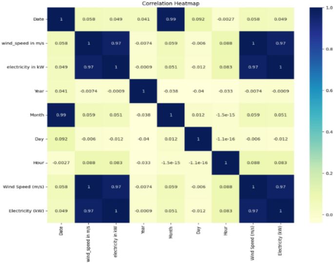
Correlation analysis of the attributes in the wind data set.
Table 1 presents a summary of the optimized hyperparameters for various machine learning models and a PINN. Each ML model is meticulously fine-tuned using fivefold cross-validation to ensure robust generalization and to mitigate overfitting to specific temporal or stochastic variations in the wind data. This cross-validation strategy facilitates the evaluation of models on multiple subsets of the dataset, thereby enhancing the reliability of performance estimates. Ensemble models, such as Random Forest, Gradient Boosting, and XGBoost, are configured with multiple estimators and regularization parameters. The tuning process for these models emphasizes capturing complex, non-linear interactions between wind features while maintaining generalization across validation folds. Simpler models, such as Linear Regression, serve as benchmarks and are evaluated using the same cross-validation protocol for consistency. The K-Nearest Neighbours model is tuned with distance-based weighting and validated across folds to more accurately model localized patterns in wind behaviour. The Neural Network architecture, comprising multiple hidden layers and employing adaptive optimization via the Adam solver, is trained and validated using Stratified K-Fold cross-validation to address non-uniform data distribution and potential class imbalance.
For the Physics-Informed Neural Network (PINN), cross-validation is adapted through a domain-specific split of the dataset into:
-
A data subdomain for supervised loss,
-
A physics-informed subdomain composed of collocation points enforcing PDE residuals, and
A validation subset is used to tune key hyperparameters such as the number of layers, neurons per layer, learning rate, and physics-constrained weighting. This structured validation ensures the PINN not only fits observational data but also adheres to the underlying physical laws governing wind energy generation. Collectively, the incorporation of cross-validation across all models strengthens the predictive rigor and ensures the hyperparameter choices yield models that generalize well to unseen wind energy data scenarios.
Data splitting
To ensure that the training set contains enough information for the model to learn patterns and that the testing set is hidden during training, the pre-processed data is randomly divided into 80% training and 20% testing subsets. This allows for an accurate assessment of the model’s generalization and predictive performance.ance44.
Figure 3 illustrates the data distribution used in the model development process. As shown, 80% of the dataset (in green) is allocated for training, while the remaining 20% (in yellow) is reserved for testing. This commonly adopted 80/20 split ensures that the model is trained on a substantial portion of the data while preserving a representative set for reliable performance evaluation and validation.
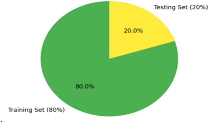
Data distribution diagram.
Evaluation
The trained models use input variables from the testing dataset to predict wind power output (Predicted Power)44. The actual power measured from the testing dataset is compared to the expected power outputs. The evaluation metrics are,
Mean absolute error (MAE):
Calculates the average size of forecast mistakes without taking direction into account.
$${varvec{M}}{varvec{A}}{varvec{E}}=frac{1}{{varvec{n}}}sum_{{varvec{i}}=1}^{{varvec{n}}}|{{varvec{y}}}_{{varvec{i}}}-{{varvec{y}}}_{{varvec{k}}}|$$
(1)
where, ({y}_{i}) is the actual value, ({y}_{k}) is the predicted value, and n is the number of samples.
Mean Squared Error (MSE):
Increases the penalty for greater mistakes by squaring them.
$${varvec{M}}{varvec{S}}{varvec{E}}=frac{1}{{varvec{n}}}sum_{{varvec{i}}=1}^{{varvec{n}}}{({{varvec{y}}}_{{varvec{i}}}-{{varvec{y}}}_{{varvec{k}}})}^{2}$$
(2)
Root Mean Squared Error (RMSE):
Stands for the average squared difference between the expected and actual numbers, squared as a root.
$${varvec{R}}{varvec{M}}{varvec{S}}{varvec{E}}=sqrt{frac{1}{{varvec{n}}}sum_{{varvec{i}}=1}^{{varvec{n}}}{({{varvec{y}}}_{{varvec{i}}}-{{varvec{y}}}_{{varvec{k}}})}^{2}}$$
(3)
R-Squared (Coefficient of Determination):
Shows how well the model accounts for the variation in the data.
$${{varvec{R}}}^{2}=1-frac{frac{1}{{varvec{n}}}sum_{{varvec{i}}=1}^{{varvec{n}}}{left({{varvec{y}}}_{{varvec{i}}}-{{varvec{y}}}_{{varvec{k}}}right)}^{2}}{frac{1}{{varvec{n}}}sum_{{varvec{i}}=1}^{{varvec{n}}}{left({{varvec{y}}}_{{varvec{i}}}-{{varvec{y}}}^{|}right)}^{2}}$$
(4)
where, ({y}^{|}) is the mean of the actual values.
In order to provide accurate wind power forecasts, this iterative process makes sure the selected model is optimized, opening the door for ongoing developments in renewable energy forecasting and optimization43.
Mathematical modelling of stacking ensemble (RF + XGB)
Let,
X= [X1, X2,……,Xn] ∈ ℝn×d be the input feature matrix.
y = [y1, y2,…….,yn] ∈ ℝn be the target values.
fRF is the function learned by the Random Forest model.
fXGB is the function learned by the Xtreme Gradient Boosting model.
fmeta is the meta-learner, trained on the outputs of RF and XGB.
Base learners Predictions:
For each sample Xi:
$$y_{i}^{{widehat{{}}(1)}} = f_{RF} (X_{i} )$$
(5)
$$y_{i}^{{widehat{{}}(2)}} = f_{RF} (X_{i} )$$
(6)
Meta-Feature Construction:
$$Z_{i} = [y_{i}^{{widehat{{}}(1)}} ,y_{i}^{{widehat{{}}(2)}} ]$$
(7)
Let Z = [Z1,….., Zn] ∈ ℝn×2
Train Meta-Learner:
The meta-learner is trained on (Z, y):
$$y_{i}^{{widehat{{}}}} = f_{meta} (Z_{i} ) = f_{meta} ([y_{i}^{{widehat{{}}(1)}} ,y_{i}^{{widehat{{}}(2)}} ])$$
(8)
fmeta is the Ridge Regression model
Wind energy simulation framework
The wind energy simulation framework, illustrated in Fig. 4, represents a comprehensive computational model that integrates all critical components of a wind power generation system to analyze and optimize energy conversion from wind resources to the electrical grid. The framework begins with aerodynamic modeling of wind turbine interactions, incorporating dynamic pitch control algorithms that continuously adjust blade angles to maximize energy capture while maintaining safety constraints across varying wind conditions. The simulation encompasses drivetrain mechanics, including gearbox efficiency, rotational dynamics, and mechanical losses during the speed conversion process from slow-rotating turbine shafts to high-speed generator inputs. The electrical conversion modeling focuses on the Permanent Magnet Synchronous Generator (PMSG) and power electronics, simulating electromagnetic interactions, voltage regulation, frequency control, and power conditioning circuits necessary for grid-compatible output. Finally, the framework incorporates grid connection modeling, which evaluates system interactions with the broader electrical network, including load balancing, power flow analysis, and considerations for grid stability. This holistic simulation approach enables engineers to predict system performance under diverse operating conditions, optimize component design and control strategies, and ensure reliable integration of renewable wind energy into existing electrical infrastructure while maintaining power quality standards and grid stability requirements.
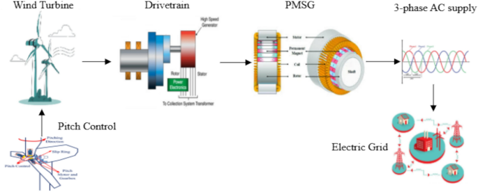
Wind Power Generation System: From Turbine to Grid—A Complete Energy Conversion and Transmission Flow Diagram.
Aerodynamic wind turbine model
The power equation to calculate the mechanical power output from wind turbine
$${mathbf{P}}_{mathbf{m}}=0.5times {varvec{uprho}}times mathbf{A}times {mathbf{C}}_{mathbf{p}}({varvec{uplambda}},{varvec{upbeta}})times {mathbf{V}}^{3}$$
(9)
where,
V- Wind speed in m/s,
Cp– Power coefficient as a function of tip-speed ratio (λ) and pitch angle (β),
ρ– Air density in kg/m3,
A-The swept area of the wind turbine blades,
Pm– Output mechanical power28.
Figure 5 illustrates the relationship between turbine output power and turbine speed across a range of wind velocities, from 5 m/s to 11.4 m/s. It shows that power generation peaks at various turbine speeds, with the base wind speed of 9 m/s achieving the maximum power. Higher wind speeds result in greater power output, but they also exhibit a more pronounced decline in efficiency as turbine speeds increase.
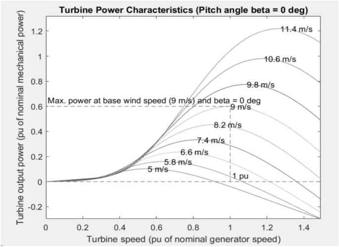
Wind Turbine Power Characteristics at Various Wind Speeds with Fixed Pitch Angle (β = 0°).
Pitch control system
Pitch control in wind turbines adjusts the angle of the blades (pitch angle) to regulate power output by minimizing mechanical stress or stopping the turbine at high wind speeds to prevent damage, while also increasing aerodynamic efficiency at low to moderate wind speeds.
-
o
At rated wind speed or higher, increase the blade pitch angle (β) to reduce Cp and limit power output.
-
o
Control law (PID control recommended)
$${varvec{upbeta}}={mathbf{K}}_{mathbf{p}}times left({mathbf{P}}_{mathbf{e}mathbf{r}mathbf{r}mathbf{o}mathbf{r}}right)+{mathbf{K}}_{mathbf{i}}times int {mathbf{P}}_{mathbf{e}mathbf{r}mathbf{r}mathbf{o}mathbf{r}}mathbf{d}mathbf{t}+{mathbf{K}}_{mathbf{d}}times frac{{mathbf{d}mathbf{P}}_{mathbf{e}mathbf{r}mathbf{r}mathbf{o}mathbf{r}}}{mathbf{d}mathbf{t}}$$
(10)
Where, ({{varvec{P}}}_{{varvec{e}}{varvec{r}}{varvec{r}}{varvec{o}}{varvec{r}}}=boldsymbol{ }{{varvec{P}}}_{{varvec{r}}{varvec{a}}{varvec{t}}{varvec{e}}{varvec{d}}}-boldsymbol{ }{{varvec{P}}}_{{varvec{m}}})45
Drivetrain model
The rotor, shaft, gearbox (if applicable), generator, and power electronics are all represented by the drivetrain model of a wind energy conversion system (WECS). Multi-mass dynamic equations are utilized to analyze torque transmission, rotational dynamics, and energy conversion efficiency, thereby optimizing performance, reliability, and fault detection in various drivetrain configurations, including geared, direct-drive, and hybrid systems.
Model the rotor, shaft, and generator dynamics. A two-mass model is commonly used:
$${mathbf{J}}_{mathbf{r}}=frac{{mathbf{d}mathbf{w}}_{mathbf{r}}}{mathbf{d}mathbf{t}}={mathbf{T}}_{mathbf{m}}-{mathbf{T}}_{mathbf{s}}$$
(11)
$${mathbf{J}}_{mathbf{g}}=frac{{mathbf{d}mathbf{w}}_{mathbf{g}}}{mathbf{d}mathbf{t}}={mathbf{T}}_{mathbf{s}}-{mathbf{T}}_{mathbf{e}}$$
(12)
where, Jr, Jg– Moment of inertia for Rotor and generator, ωr, ωg– Angular velocities for Rotor and generator, Tm– Mechanical torque from the turbine, Ts– Shaft torque, Te– Electrical torque generated from the generator46.
Generator model (PMSG)
The electrical and mechanical dynamics of a wind energy conversion system (WECS) are represented by the Permanent Magnet Synchronous Generator (PMSG) model.
Permanent magnets on the rotor improve efficiency and reliability by removing the need for an external excitation system, and the system is controlled by electromagnetic equations in the dq-reference frame, which are expressed as follows:
$${mathbf{V}}_{mathbf{d}}={mathbf{R}}_{mathbf{s}}{mathbf{I}}_{mathbf{d}}+{mathbf{L}}_{mathbf{d}}frac{mathbf{d}{mathbf{I}}_{mathbf{d}}}{mathbf{d}mathbf{t}}-{varvec{upomega}}{mathbf{L}}_{mathbf{q}}{mathbf{I}}_{mathbf{q}}$$
(13)
$${mathbf{V}}_{mathbf{q}}={mathbf{R}}_{mathbf{s}}{mathbf{I}}_{mathbf{q}}+{mathbf{L}}_{mathbf{q}}frac{mathbf{d}{mathbf{I}}_{mathbf{q}}}{mathbf{d}mathbf{t}}+{varvec{upomega}}{mathbf{L}}_{mathbf{d}}{mathbf{I}}_{mathbf{d}}+{varvec{upomega}}{{varvec{uplambda}}}_{mathbf{m}}$$
(14)
$${mathbf{T}}_{mathbf{e}}=frac{3}{2}mathbf{P}({{varvec{uplambda}}}_{mathbf{m}}{mathbf{I}}_{mathbf{q}}+({mathbf{L}}_{mathbf{d}}-{mathbf{L}}_{mathbf{q}}){mathbf{I}}_{mathbf{d}}{mathbf{I}}_{mathbf{q}})$$
(15)
where, Vd, Vq– stator voltages, Id, Iq– stator currents, Rs– stator resistance, Ld, Lq– stator inductances, λm– flux linkage from permanent magnets, ω- electrical angular velocity, Te– electromagnetic torque, P- number of pole pairs. This model supports control algorithms that maximize wind energy conversion while preserving grid stability and dynamic performance, such as Field-Oriented Control (FOC) and Maximum Power Point Tracking (MPPT)47. Table 2 shows the values of the blocks used in building the wind energy conversion system model in MATLAB Simulink. Figure 6 illustrates a comprehensive wind turbine control system modeled in Simulink, incorporating a Permanent Magnet Synchronous Generator (PMSG) with electromagnetic torque feedback loops and wind speed inputs to optimize power generation performance. The system integrates key components, including pitch angle control, drive train dynamics, generator speed regulation, and the conversion of mechanical energy into a three-phase AC electrical output.
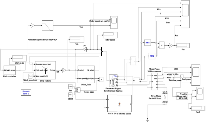
PMSG-Based Wind Turbine Control System with Drive Train and Pitch Control using predicted wind speed from the ML models.
Physical informed neural network (PINN)
A Physics-Informed Neural Network’s (PINN) core architecture and operational process are depicted in Fig. 7. Physical inputs are received by the neural network, which translates them into output variables. It is composed of an input layer, several hidden layers, and an output layer. In contrast to traditional neural networks, PINNs use a loss function that blends differential equation loss with physical constraint loss to incorporate physical information. This ensures that the anticipated results comply with the governing physical laws, in addition to aligning with the training data. The weights and biases are finalized when the overall loss drops below a predetermined tolerance, which is achieved by continuing the training cycle. By bridging the gap between physics-based systems and data-driven models, this hybrid learning technique makes PINNs ideal for intricate scientific and engineering applications.
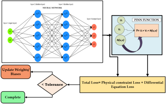
Workflow of a Physics-Informed Neural Network (PINN) for Solving Physical System Constraints.
Mathematical modelling of PINN
To model electricity generation (widehat{P}left(tright)) From wind energy using a neural network that:
-
Learns from real-time measurements
-
Obeys physical constraints (from simulation)
-
Enforces power-wind relationships and turbine characteristics
-
Inputs and features
Let,
v(t)= Wind speed at time t (from real data)
θ(t)= Pitch angle (from simulation)
wr(t)= Rotor speed (from simulation)
Tm(t)= Mechanical torque (from simulation)
Te(t)= Electrical torque (from simulation)
X(t)∈ℝd= Complete feature vector including time-based cyclic features
$$Xleft( t right), = ,[vleft( t right),theta left( t right),w_{r} left( t right), , T_{m} left( t right), , T_{e} left( t right), , sin (frac{2Pi Month}{{12}}), , cos (frac{2Pi Month}{{12}}), ldots ..]$$
(16)
fθ= Neural network with parameters θ
(widehat{P}left(tright))= Predicted electrical power output at time t.
Where,
V- Wind speed in m/s,
Cp– Power coefficient as a function of tip-speed ratio (λ) and pitch angle (β),
ρ– Air density in kg/m3,
A-The swept area of the wind turbine blades,
Pm– Output mechanical power. Using Betz’s limit,
$$P_{expected} left( t right), = ,eta times P_{m} (t)$$
(19)
Typical efficiency= 0.6
-
Constraint: Predicted power must not exceed expected power
$$Lefficiency = frac{1}{N}sumnolimits_{(i = 1)}^{N} {[max (0,hat{P}(t_{i} ) – eta times P_{m} (t_{i} ))]^{2} }$$
(20)
-
Cut-in, rated, and cut-out constraint
Cut- in speed Vin= 3 m/s
Rated speed Vrated= 9 m/s
Cut- out speed Vout= 25 m/s
η(V) = (left{begin{array}{c}0 V< {V}_{in} or V> {V}_{out}\ 1 otherwiseend{array}right.)
Constraints:
$$Lcutoff = frac{1}{N}sumnolimits_{(i = 1)}^{N} {[hat{P}(t_{i} ) times } (1 – eta (V_{i} )]^{2}$$
(21)
From physics and simulation:
$$P_{sim} (t) = w_{r} (t) times T_{e} (t)$$
(22)
So enforce:
$$L_{s} im = frac{1}{N}sumnolimits_{(i = 1)}^{N} {(hat{p}(t_{i} )} – P_{s} im(t_{i} ))^{2}$$
(23)
αi- Tunable weights for each physical constraint.
Dataset configuration for PINN model evaluation
This section outlines the comprehensive dataset strategy employed for PINN model evaluation, which leverages a dual-source data approach to maximize both empirical accuracy and physical consistency. The evaluation framework employs a hybrid data integration strategy to train and validate the PINN model by combining real-world and simulation-based datasets. The real-time MERRA-2 dataset (Case 1) provides globally consistent meteorological inputs, including date, time, wind speed, and electricity generation (in kW). To complement this, a synthetic dataset is generated through MATLAB-based physical simulations (Case 2), where partial differential equations governing wind turbine aerodynamics and electromechanical behavior are used to compute critical operational parameters such as pitch angle, rotor speed, mechanical torque, electrical torque, and generated power. By integrating these two data sources, the PINN model can simultaneously learn from empirical observations and the governing physical laws of wind energy conversion. This approach ensures that predictions are not only data-driven but also physically consistent, effectively capturing the complex, real-world dynamics essential for accurate and reliable wind power forecasting.
Table 3 presents the performance analysis across varying wind speeds, illustrating the characteristic operational behaviour of wind turbines under different atmospheric conditions and revealing distinct performance zones based on wind velocity. At the above-rated wind speed of 14 m/s, the turbine operates with active pitch control (1.072 p.u) to regulate power output, achieving high rotor speed (153.1 rad/s), near-optimal mechanical torque (0.9979 Nm), substantial electrical torque (64.2 Nm), and maximum electricity generation (9788.98 W). The rated wind speed condition of 9 m/s represents optimal operation, where the turbine maintains efficient performance with zero pitch angle adjustment, a good rotor speed (133.3 rad/s), moderate mechanical torque (0.7216 Nm), and a substantial power output (7386.1 W). In contrast, the below-rated wind speed scenario of 6 m/s illustrates sub-optimal operation where the turbine experiences reduced efficiency with minimal mechanical torque (0.2531 Nm), lower rotor speed (95.48 rad/s), and significantly decreased electricity generation (3806.93 W), highlighting the direct correlation between wind speed availability and turbine performance parameters across the operational envelope. The analysis reveals that electricity generation varies dramatically with wind speed, following the cubic relationship P ∝ V3, where power output increases from 3806.93 W at 6 m/s to 9788.98 W at 14 m/s. This demonstrates how wind velocity directly governs energy conversion efficiency, making accurate wind resource assessment critical for reliable renewable energy planning and grid integration.