Surface appearance of poly lactic acid due to variations in material extrusion processing parameters

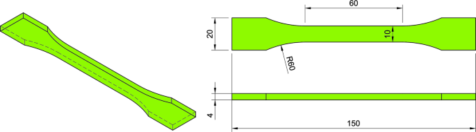
The total number of PLA specimens generated was 17, with k = 3 and C_o = 5. The developed DoE plan is shown in Table 3.

All MEX specimens were in good condition; no layer delamination, warping, or material degradation was detected. However, as Fig. 6 shows, the color difference and surface aspects between specimens of different sets were evident through a simple visual inspection. The variations in process parameters caused the color difference. It was perceptibly apparent that the white-black shift and intensity increased with the permanence time of the material in the melt condition and the raster dimensions. As expected, a low deposition time was associated with thicker material accumulation, resulting in a well-defined deposition raster with a smaller width. The peaks of each raster had higher gray values than the surrounding valleys. On the contrary, the rasters realized with high deposition were thinner, with a larger width, and exhibited minor variations between peaks and valleys.

Root mean squared height S_q and arithmetical mean height S_a were the metrics used in MountainMap to measure the surface texture, as they were not sensitive to measurement parameters such as sampling length and evaluation length²⁸. S_q represented the root mean square of ordinate values within the defined ROI of area A, equivalent to the root mean square deviation R_q. S_a was the extension to the surface of a line’s arithmetical mean height R_a, expressing, as an absolute value, the difference in height of each point compared to the arithmetical mean of the surface. These parameters were generally used to evaluate surface roughness. The expressions S_q-Z and S_a-Z are reported below, where the subscript Z is associated with the LBCH acquisition.

The color of the specimen surface was quantitatively analyzed with Fiji and then transferred to MountainMap. Black had the lowest intensity, and white had the highest. The color is assumed to be 0 for black and 255 for white. The intensity data of each specimen was measured at each point of the image, generating an XYG cloud in which X and Y are the spatial coordinates, and G is the associated grey value. In the case of image analysis, the Z value was substituted with the G value, and the expressions S_q-G and S_a-G are

Table 4 reports the results of the Conoscan and Fiji measurements. The value variations of all response variables were significant, pointing out the MEX process’s sensitivity to the process parameters.

The analysis of variance (ANOVA) was performed using designexpert (Stat-Ease inc., minneapolis, USA). the degree of freedom (df), the sum of squares (SS), mean square (MS), fisher’s value (F-value), and probability value (p-value) of each response are reported in Tables 5, 6, 7 and 8. the model was significant for all responses, with p-values ranging from 0.0010 to 0.0017. the flow rate Q was the most influential factor, followed by the nozzle temperature T_n and the fan speed F. the investigation of the ANOVA results gave an essential overview of the statistical model to use. According to the analyses of all responses, the linear model was significant, and the lack of fit was not substantial relative to the pure error. there was a high chance that the lack of fit could occur due to noise. the coefficient of determination R² was higher than 67%, and the adq precision ratio was greater than 9.7, suggesting that the linear models were suitable for exploring and optimizing the design space

The Response Surfaces of S_q and S_a metrics are reported in Figs. 7 and 8 for the Conoscan and Fiji acquisitions.

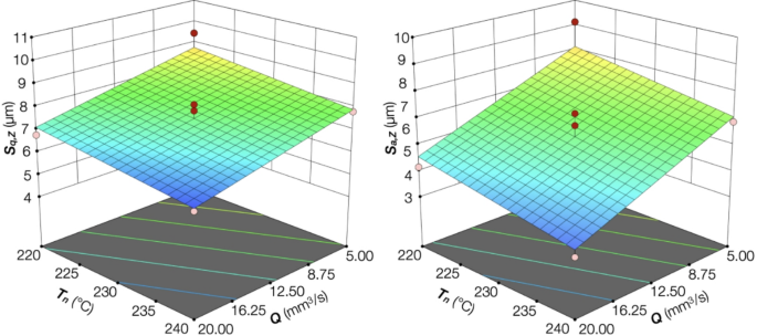
Conoscan surface metrics with F = 75%.

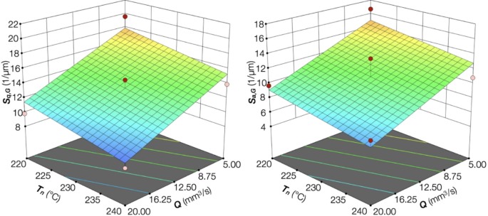
Fiji surface metrics with F = 75%.

The results trends of both acquisition systems were the same for the two responses. The S_q and S_a values decreased with increased flow rate Q and nozzle temperature T_n. The contrary happened with increased flow rate Q and nozzle temperature T_n. The decrease in fan speed F caused the S_q and S_a values to be slightly reduced. The framework for the grayscale gave the same trends as the laser-based method. The primary advantage was the processing speed, which made this method suitable for online measurements.

The specimens with ID 5 (Q = 20 mm³/s, T_n = 240 °C, and F = 75%) and ID 15 (Q = 5 mm³/s, T_n = 220 °C, and F = 75%) were selected to compare the surface morphology, representing two opposite sets, respectively, with the lowest and the highest values of the surface metrics. Figure 9 shows the 5 × 5 mm² ROI of the investigated samples and the computed 3D surface topography, filtered using a Gaussian low-pass filter with a cutoff of 0.8 mm. The surface with the lowest peak heights was associated with specimen ID 5, indicating that the process parameter set used for this specimen was the best option for achieving a maximum peak height of 5 μm. The minimum error was also achieved, primarily due to the solidification conditions after deposition. The effect of the flow rate and nozzle temperature on roughness was notably more substantial than that of fan speed. On the contrary, the surface peak heights were higher for sample ID 15, reaching the maximum value of 20 μm. Moreover, the deposition rasters on the surface were more evident, with an apparent alternation between peaks and valleys. Significant differences were not found between trends of Conoscan and Fiji elaborations. The peaks and valleys of Fiji elaboration had values different from those of Conoscan, but the trends remained the same. The lower precision resulted in a coarser granularity of the Fiji surface reconstruction compared to the Conoscan resolution.

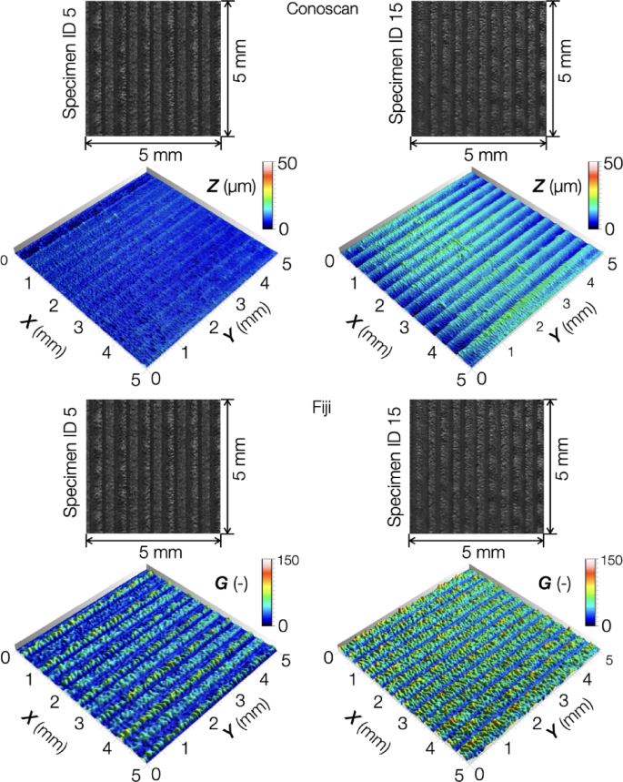
Surface of specimen ID 5 and ID 15.

The next step was to analyze the distribution of the gray value using a histogram curve. This graph displays the frequency of points with a given gray value height for specimen IDs 5 and 15, as reported in Fig. 10, working on Fiji surfaces.

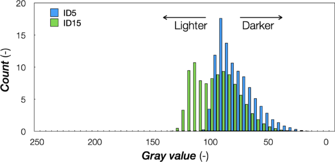
Fiji Histograms of specimen ID 5 and ID 15.

The shape of the frequency distribution was very interesting to evaluate. ID 5 was positively skewed (not symmetrical), with the longer distribution tail occurring for higher values of the measured variable, revealing that the mean, median, and mode were unequal. The symptom was associated with a smaller width of the deposition rasters with the parameter set. The regular alternation of peaks and valleys in ID 15 generated a bimodal distribution, with valleys darker than the peaks. From these observations, product surface roughness errors could be monitored, and the effects of the related process parameters could be recognized and adjusted to mitigate possible defective parts through closed-loop feedback control.

The mechanical tests were lastly performed on all specimens. The initial cross-section of each specimen was measured before testing using a digital micrometer. The maximum strain ε established for each test was 20%. All specimens broke in a fragile manner, considering the absence of a plateau after the yield point, with a low-stress drop (Fig. 11). Moreover, the elongation and tensile toughness values (as indicated by the area under the stress-strain curve) were higher than those specified in the material data sheet. Table 9 lists the tensile properties of the printed specimens, including Young’s modulus E, Tensile strength σ_R, and Strain at break ε_tb. A portion of the stress-strain curves between 5 and 20 MPa was used for the modulus calculations. The low value of 5 MPa was needed to achieve load stabilization during testing for all involved rasters. The mechanical test results revealed that the variation of response variables was more significant than 5% but lower than 10%, indicating the test repeatability compared to the median value. The stress-strain curves were reported to highlight the repeatability of the performed tests and were then analyzed statistically. The subplots of each response variable were also shown in the same figure. The degree of freedom (df), the sum of squares (SS), mean square (MS), Fisher’s value (F-value), and probability value (p-value) of each response of the ANOVA are reported in Tables 10, 11 and 12. The model was significant for all responses, with p-values ranging from 0.0002 to 0.0063. The flow rate Q was the most influential factor for E and ε_tb, while the fan speed F was the most important for σ_R.

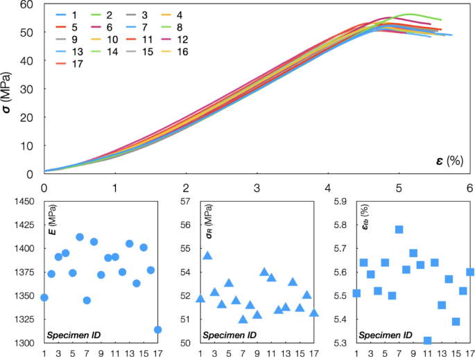
Tensile test results with F = 75% and Q = 12.5 mm³/s.

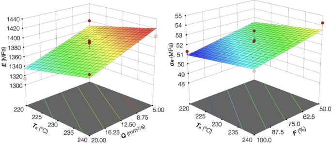
The Response Surfaces of E and σ_R metrics are reported in Fig. 12 for tensile test results. The specimens with IDs 13 (Q = 5 mm³/s, T_n = 240 °C, and F = 75%) and 17 (Q = 20 mm³/s, T_n = 220 °C, and F = 75%) were selected to compare their mechanical responses, representing the two sets with the lowest and highest mechanical responses. The value of the Young modulus confirmed the high performance of the specimen with ID 13 compared to the specimen with ID 17. However, the variations of σ_R and ε_tb of the two specimens were low, indicating the stability of the other mechanical responses to variations in the process parameters. For this reason, the comparison was extended to the specimens with ID 5 (Q = 20 mm³/s, T_n = 240 °C, and F = 75%) and ID 15 (Q = 5 mm³/s, T_n = 220 °C, and F = 75%), which were previously analyzed for their response to the surface metrics. For the specimen with ID 5, the E, σ_R, and ε_tb values fell within the median values, even if the surface metrics were the lowest. This behavior was justified by the consistently high raster density, which resulted in high adhesion between the printed layers, making the structure denser and thereby increasing its strength. On the contrary, the specimen with ID 15 was characterized by the lowest σ_R and ε_tb values, while the E value was the highest. The reason was to re-examine the raster configuration, which improved the specimen’s stiffness.

The analysis of the relationship between surface metrics (S_a and S_q) and mechanical properties (E, σ_R, and ε_th) was also performed. The scatter plots in Fig. 13 display the mechanical values as a function of the surface roughness values, with each point on the graph representing a single data observation. The data points for all graphs were randomly dispersed across the plot, and no discernible pattern or trend was detected. The linear regression coefficients ranging from 0.1 to 0.25 suggested the absence of a relationship between the examined variables and a large dispersion of points. The reason for this result was justified by the fact that the mechanical resistance was more influenced by the inner specimen structure (infill pattern and density) with respect to the outer surface quality²⁹.

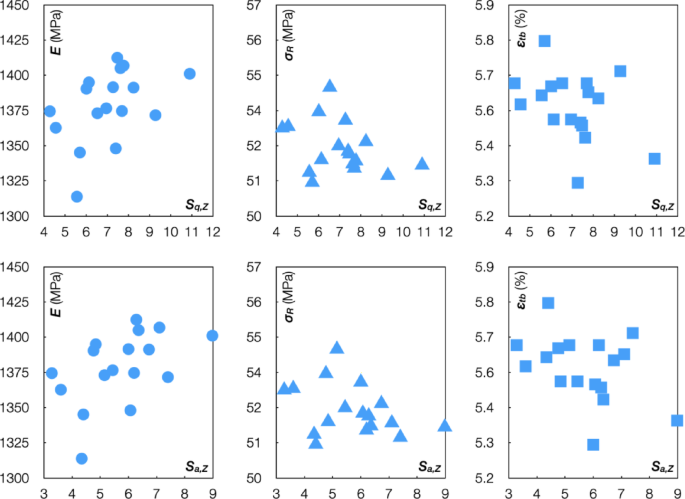
Correlation graphs between surface metrics and mechanical performance.