Some suggested ARIMA models and Bayes estimates for real-world time series data sets are numerically illustrated in this section. The example serves as a key demonstration of how our models work in finding a true state of the system by showcasing the method’s practical utility and relevance to real-life problems. In addition to the analysis, we have also mentioned the forecast for future purposes.
Data source
We have taken a real data set of the IMR for India over the period of 73 years from 1950 to 2023 annually. The data set is given in the form of a time series from World Population Prospects. World Population Prospects is the twenty-seventh edition of official United Nations population estimates and projections that have been prepared by the Population Division of the Department of Economic and Social Affairs of the United Nations Secretariat. It presents population estimates from 1950 to the present for 237 countries or areas underpinned by analyses of historical demographic trends. This latest assessment considers the results of 1,758 national population censuses conducted between 1950 and 2023, as well as information from vital registration systems and 2,890 nationally representative sample surveys (UN-WPP). Table 2 shows the IMR values, and Table 3 shows the IMR growth rate in percentage.
After understanding the dataset, we have drawn the time series plot of IMR growth rate data and differenced IMR growth rate. These plots are given in Fig. 1.
Time series plots showing IMR growth and differenced IMR growth rate of India from 1951-2023
After plotting the IMR growth data, it can be observed that it is not stationary (see Fig. 1a). However, after differencing it once, we obtain stationarity in Fig. 1b. This shows that we can set (d=1). The ADF test also shows that unit root is not present for the first difference. The p-value (=0.31) is also greater than 0.05.
ACF and PACF plots for the given data
Selecting the appropriate values for p and q is crucial in building an effective ARIMA model for a given time series [7]. To determine p and q, we have drawn the ACF and PACF plots as mentioned in Determining the order section. This plotting involves computing the autocorrelation function (ACF) and partial autocorrelation function (PACF) plots of the time series data. ACF is a plot of the correlation of a series with its own lagged values. PACF plot is a plot of the partial correlation between a series and its lagged values, regressed the values of the time series at all shorter lags. ACF and PACF plots of the data are given in Fig. 2.
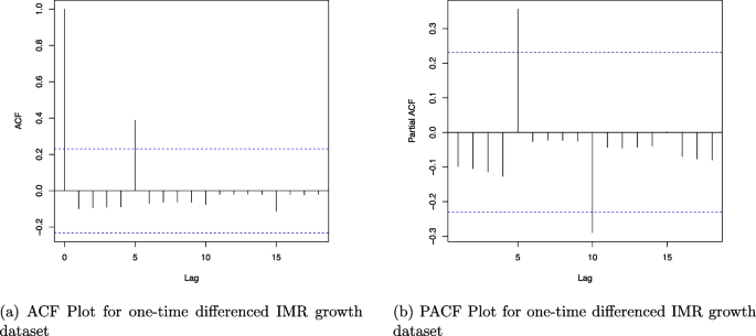
ACF and PACF plots of the IMR growth dataset after first differencing
The above ACF (see in Fig. 2a) and PACF plots (see in Fig. 2b) are shown with details. Significant autocorrelation spikes at specific lags may indicate periodic behaviour or a strong dependence on past values, as seen at lag 5, which is the highest. Significant spikes at multiple lags may suggest a mix of autoregressive and moving average components, indicating a more complex time series structure in the partial autocorrelation at lags 5 and 10, respectively. Furthermore, these plots provide valuable insights into the temporal dependencies within a time series, aiding in model selection and forecasting. Using all the nearest possible combinations of AR lag, fixing the difference at one time, and other nearest lag possible combinations of MA order, we go for the likelihood estimation and Bayesian estimation as well in the next section.
Classical analysis
The primary aim of the study is to emphasise Bayesian analysis, a crucial aspect of establishing initial values to compute the MLE using the Newton-Raphson method. This initial value helps us to run the algorithm 3.4. In this study, the ARIMA model results from the specified combinations of (p, d, q), namely (5,1,0), (5,1,1), (5,1,2),(5,1,3),(5,1,4),(5,1,5), (0,1,5), (1,1,5), (2,1,5),(3,1,5), (4,1,5) and (5,1,5). Since we have stationarity at the first lag, we have selected d = 1. Although the ACF and PACF plots suggest a lag of 5, we are not very sure about it. Therefore, we have selected these combinations of p and q. We have computed the MLE for the mentioned models, along with their respective standard errors (SE), for the above-selected combinations of p and q in the ARIMA (p, d, q) model, and their AIC and BIC values. The results are shown in Table 4.
From Table 4, it can be seen that the ARIMA models generally show consistent parameter estimates across different parameter specifications, with varying degrees of uncertainty (as indicated by the standard error, SE). Notably, the order (5,1,0) and (0,1,5) models have more stable parameter estimates with relatively lower standard errors compared to higher-order models like (5,1,3), (5,1,4), (5,1,5), where standard errors are larger, indicating less precise estimates. Additionally, the ARIMA models with moving average terms (e.g., order (5,1,1) and (5,1,2)) show slightly higher parameter variability, suggesting increased model complexity that may lead to poor precision.
Besides classical estimates, Table 4 presents AIC and BIC values. Based on these values, we can say that ARIMA models with orders (5,1,0), (5,1,1), (0,1,5) and (1,1,5) are performing better than the others. Also, it is well known that Bayesian analysis is computationally costly, due to the need for repeated likelihood evaluations and high-dimensional sampling using Markov Chain Monte Carlo (MCMC) methods. Each iteration of the Random Walk Metropolis algorithm requires evaluating the full likelihood via the Kalman filter, which increases computational load significantly. Therefore, to ensure tractability and focus on the most promising configurations, we restrict the Bayesian analysis to four models that showed the best performance in the classical model selection phase. Therefore, we plan to perform a Bayesian analysis for these four models only. In the next subsection, we will provide the Bayesian analysis of these four models.
Bayesian analysis
To conduct Bayesian analysis, the initial step involves determining the prior hyperparameters. Since the Bayesian framework relies heavily on prior information, carefully selecting priors is crucial to avoid misleading results. As suggested in Prior distribution section, the most appropriate prior for both the (phi) and (theta) parameters is the Multivariate Normal (MVN) distribution. We choose the hyperparameters as follows: The MLE (hat{phi }) of ({phi }) is considered as the prior mean for the respective AR models. The diagonal elements of the prior variance-covariance matrix (Sigma) is 2(times) abs [({phi _1}), ({phi _2}),…, ({phi _5})]. The non-diagonal elements of (Sigma) are considered to be zero. In the same way, we choose the MLE and diagonal elements of the prior variance-covariance matrix for the (theta) parameter of the MA model (details mention in 3.2).
We now proceed to run the RWM algorithm, as discussed in Random walk Metropolis (RWM) algorithm section. The proposal scale, (sigma), has been chosen in the algorithm to keep the acceptance rate optimal. The initial values of the chain are set to the corresponding MLE. The algorithm has been run for 5e5 iterations. Under the aforementioned conditions, the optimal acceptance rate ranged from (10%) to (60%), indicating a low rejection rate of the algorithm.
Table 5 presents estimated posterior characteristics for different configurations of the models, which have been chosen according to the minimum AIC and BIC values. So, we have chosen four models of order (5,1,0). (5,1,1), (0,1,5), (1,1,5). The posterior summary includes the posterior mean, median, mode, and highest posterior density (HPD) intervals with a 0.95 probability.
By varying the hyperparameter of prior distributions and comparing the resulting posterior summaries, we observed that the estimates remained largely consistent, indicating robustness of the Bayesian inference. Across the models, the parameter estimates indicate variability in both magnitude and uncertainty. In general, the fifth lag of the AR or MA terms shows relatively larger means and wider HPD intervals, suggesting a stronger or more uncertain contribution at that lag. Comparing models, the ARIMA(5,1,1) and ARIMA(1,1,5) appear to capture richer dynamics due to the inclusion of both AR and MA terms, although some parameters show wide HPD intervals, implying caution in their interpretation.
From Fig. 3 shows the trace plots from 5e5 MCMC iterations show well-mixed, stationary chains for all five parameters, with no visible trends or drifts. The rapid fluctuations indicate low autocorrelation, suggesting good convergence and reliable posterior sampling. This analysis helps identify the most suitable model structure for forecasting while highlighting parameter uncertainty. Further details of this combination of models has been discussed in the next subsection.
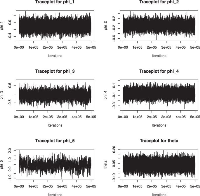
Trace plot of the parameters for order (5,1,1)
Bayesian model selection
In order to proceed with model selection, which is to make a comparison among models, and wish to know the best one among four models considered for Bayesian Analysis. We have used the AIC score, BIC score for model selection as discussed in Bayesian Model selection section. Also, K-fold cross-validation (CV) is used to assess the predictive performance of the selected models on simulated time series data. For practical compatibility, K is commonly set to 5 or 10; this study chose K = 10, following [34]. The results are shown in Table 6.
The Table 6 presents a comparative analysis of four Bayesian ARIMA model configurations (5,1,0), (5,1,1), (0,1,5), and (1,1,5)—based on evaluation metrics such as AIC, BIC, MSE, RMSE, and MAE. Among them, the ARIMA(5,1,0) model demonstrates the best performance, having the lowest AIC (18.68), BIC (30.14), and the most favorable error values (MSE = 4.72, RMSE = 2.17, MAE = 1.66). To provide a more comprehensive evaluation of model performance, we also computed Root Mean Square Error (RMSE) and Mean Absolute Error (MAE) for each selected ARIMA model. These metrics offer additional insight into forecast accuracy, with RMSE being sensitive to large errors and MAE providing a more robust view of average forecast deviations. The ARIMA(5,1,0) model outperforms the others across all four criteria—AIC, BIC, RMSE, and MAE—reinforcing its status as the most reliable model for forecasting India’s IMR growth.
However, ARIMA(5,1,0) offers several additional advantages that justify its selection. First, it has a simpler structure with fewer parameters than ARIMA(1,1,5) or ARIMA(0,1,5), which reduces the risk of overfitting and enhances model interpretability. Second, in the Bayesian estimation process, the ARIMA(5,1,0) model demonstrated better convergence diagnostics (e.g., well-mixed trace plots and stable posterior distributions), indicating numerical stability and robustness. These practical and computational considerations, along with its marginally better predictive accuracy, make ARIMA(5,1,0) the most appropriate model for forecasting India’s infant mortality rate in this study.
Retrospective study
This retrospective study examines the trend in interval estimates over the period 2015 to 2023. The intervals represent credible intervals, reflecting changes observed year-over-year. By systematically analysing these intervals, the study aims to understand the longitudinal behaviour of IMR growth rate, offering insights that may support future forecasting or decision-making.
The Table 7 presents forecasted IMR growth rates from 2015 to 2023, each accompanied by a 95% confidence interval. While the predicted values consistently show a decline in IMR growth( in %) over time, the widening confidence intervals (CI), especially in later years, indicate increasing uncertainty in the forecasts. This suggests that although the model anticipates continued improvement, the reliability of long-term predictions decreases as the forecast horizon extends.
Again, for validating the model’s accuracy and reliability we are comparing the forecasted IMR growth rates and their confidence intervals with actual observed data is essential. It shows how well the model reflects real trends, whether its uncertainty estimates are appropriate, and helps identify over or underestimations. This comparison also supports model refinement and builds credibility, making the forecasts more meaningful for evidence-based decision-making.
The Table 8 compares actual and forecasted IMR values from 2015 to 2023, along with the absolute error for each year. The results show that the model consistently overestimated IMR across all years, with forecasted values slightly higher than actual figures. While the forecast closely matched actual IMR in 2015 (smallest error: 0.22), the accuracy gradually declined over time, reaching the highest discrepancy in 2023 (1.51). This pattern suggests the model performs better for short-term predictions, but its accuracy diminishes as the forecast horizon extends. Overall, the model demonstrates a reasonable fit, though its tendency to over-predict should be noted for future refinement.
Comparing predictive performance
As the purpose of this article is to forecast the IMR growth data using a Bayesian ARIMA model. But for the simplicity of this study, we can go for the Autoregressive(AR) model to predict the same dataset. And also make a comparison of the predictive performance between the common forecasting model and the Bayesian ARIMA model. Since, AR models are ideal for small, stationary datasets, capturing temporal dependence through past values. They’re simple, interpretable, and effective for short-term forecasts, requiring no external inputs.
Bayesian ARIMA provides probability distributions for forecasts, and also requires a more iterative process to find the estimates. Bayesian ARIMA offers enhanced precision by incorporating uncertainty and adaptability. The choice between the two depends on the complexity of the dataset and the need for probabilistic forecasting. To evaluate the comparative performance of the two models, we present Table 9, which reports the IMR values and their growth rates for the same year, along with the corresponding 95% CI for both the AR model and the Bayesian ARIMA model.
The Bayesian ARIMA model demonstrates superior forecasting performance compared to the AR model, as shown by significantly lower MSE values averaging 4.3 across 10 folds versus 18.5 for the AR model. Also, its ability to provide probabilistic confidence intervals enhances its reliability in uncertain environments. Compared to the AR model, Bayesian ARIMA delivers more accurate and informative forecasts, especially when accounting for uncertainty and evolving data patterns.
Forecasting
To fulfil the second objective of our study, we have generated forecasts for the subsequent periods based on the fitted time series model. The model captured the underlying patterns and trends in the historical data, and the forecasted values provide an estimate of the expected behaviour moving forward. The result of the point forecast for IMR and IMR growth (in %) with their respective credible interval are summarised in Table 10 for the next decade.
To obtain these patterns, we initially simulated the corresponding posterior and obtained a posterior sample of size 1e5 for the ARIMA(5,1,0) model using available data values. Subsequently, we simulated predictive samples for the remaining unobserved datasets for each value in the simulated posterior sample. The predictive estimates are provided as the corresponding posterior modes based on 100 predictive samples. These samples are used to apply the Kalman filter to predict future observations by using the model’s estimated parameters and current state information.
The forecasted IMR from 2024 to 2033 in Table 10 indicates a consistent downward trend, highlighting gradual improvements in infant mortality rates (IMR). Starting from an IMR of 25.21 in 2024, the rate steadily declines to 15.68 by 2033. The year-over-year growth rate remains negative throughout the period, with the highest reduction observed in 2033 (-5.81%). The output typically includes forecasted values along with their associated uncertainties, which helps with short-term time series prediction.
From Fig. 4 shows that the trend is promising as this persistent decline reflects the potential impact of public health interventions, improved healthcare services, and socio-economic development. The model effectively captures this trend, offering valuable projections for health policy planning and evaluation.
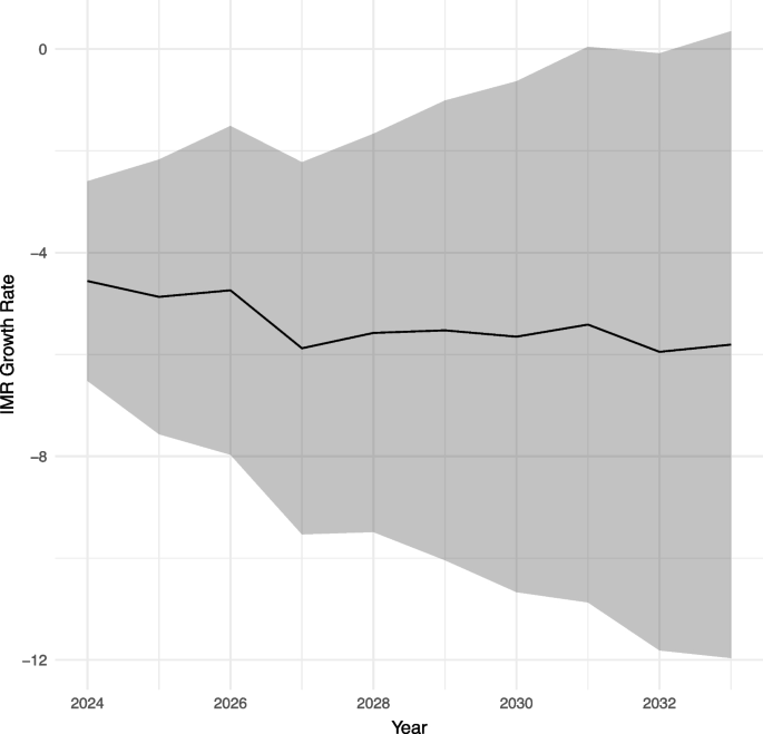
Forecasted IMR growth trend with credible intervals