Regulation of heterosis-associated gene expression complementation in maize hybrids | Genome Biology

Plant genetic resources

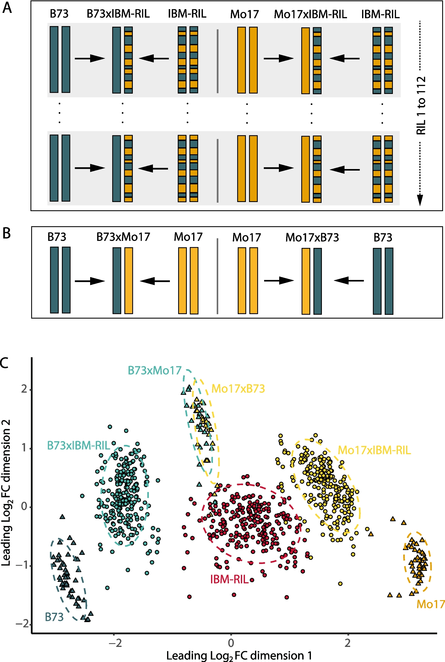
The IBM-RIL syn. 4 population [19] represents a collection of highly diversified genotypes with respect to the genomic regions contributed by their two parental inbred lines B73 and Mo17 (Fig. 1A). To study the phenotypic and transcriptomic plasticity of maize F₁ hybrids relative to their parents, a random subset of 112 IBM-RILs was backcrossed to their original parental inbred lines B73 and Mo17. In all crosses, B73 and Mo17 were selected as the female parent to secure a homogenous phenotype of all plants on which the pollinated ears will develop and thus similar seed quality. Each of the two F₁-backcross hybrids of a specific IBM-RIL (hereafter named B73 × IBM-RIL and Mo17 × IBM-RIL backcross hybrids) show contrasting homozygous and heterozygous genomic regions and genes (Fig. 1A). For example, if a region between two recombination breakpoints is homozygous in a B73 × IBM-RIL backcross, it is heterozygous in the corresponding Mo17 × IBM-RIL backcross hybrid and vice versa.

Experimental design

We studied the phenotypic and transcriptomic plasticity of the IBM-RIL backcross hybrids relative to their parental inbred Lines. A selection of 112 IBM-RILs was used as paternal inbred Lines, corresponding to 112 B73 × IBM-RIL and 112 Mo17 × IBM-RIL backcross hybrids (Fig. 1A). To optimally fit the experimental design and increase the precision of subsequent pairwise comparisons with the common parental inbred lines and reference hybrids, both common maternal inbred lines B73 and Mo17 and the two reference hybrids B73 × Mo17 or Mo17 × B73, respectively, were included (Fig. 1B). For each sample, 25 kernels of the same genotype (parent or hybrid) were surface sterilized in 10% H₂O₂ for 20 min, rinsed with distilled water and afterwards pre-germinated in filter paper rolls with five kernels each in a climate chamber with a 16 h light (26 °C), 8 h dark (21 °C) cycle in distilled water [13]. After 3 days, eight seedlings per genotype with approximately the same length of primary root and, if already present, shoot length were selected and transferred into a row of an aeroponic growth system for 4 additional days. Each aeroponic growth system (“Elite Klone Machine 96,” TurboKlone, USA) was composed of 12 rows each with eight planting sites. Thus, we could fit 12 different genotypes into one aeroponic growth system and eight systems at the same time into our climate chamber (16 h Light, 26 °C; 8 h dark, 21 °C; Additional file 1: Fig. S9). We analyzed three independent biological replicates, each comprising all IBM-RIL inbred lines and hybrids. Due to the large number of samples and space limitations, the different genotypes of each biological replicate were grown in four batches distributed across four weeks, also called alpha-design with incomplete blocks [34]. Within each batch, the eight aeroponic growth systems were randomly assigned to eight positions in the climate chamber. Three successive rows of an aeroponic growth system represent one triplet. To each triplet, an IBM-RIL and its corresponding B73 and Mo17 backcross hybrids, or both common maternal inbred lines B73 and Mo17 and one of the two reference hybrids B73 × Mo17 or Mo17 × B73, respectively were assigned. The randomization process was conducted at the replicate level for the triplets, whereas it was ensured that in each batch two reference triplets each of B73, Mo17, B73xMo17 and B73, Mo17, Mo17xB73 were distributed. Thus, in each batch, we surveyed 30 IBM-RIL triplets and both reference hybrids and the common inbred lines B73 and Mo17 in two additional triplets (Additional file 1: Fig. S9). So that in total, 3 samples of each IBM-RIL and each backcross hybrid, 48 samples (biological replicates) of the maternal inbred lines B73 and Mo17, and 24 samples of the reciprocal hybrids B73 × Mo17 and Mo17 × B73 as reference hybrids were analyses. In other words, each independent biological replicate contained 384 samples (in total: 384 × 3 replicates = 1152 samples). The number of individual samples per replicate was designed to also fit one sequencing run on the NovaSeq 6000 S4 flow cell machine (Illumina, San Diego, USA), described later.

Root phenotyping and sampling for RNA-seq

Seven days after germination, all seedlings per sample (maximum eight seedlings) were removed from the aeroponic growth system, and the seedling root system was scanned using an Epson Expression 12000XL scanner (Epson, Meerbusch, Germany) with up to four plants per image. The resulting images were cropped to create single plant images that only showed the root system and the maize kernel. We used the RootPainter software client (version 0.1.0) and server component (version 0.2.7) to train a convolutional neural network to recognize and segment roots in images [35]. We then analyzed the segmented images in a batch using RhizoVision Explorer (version 2.0.3) [36]. After inspection and cleanup, we determined the total root length, the total root volume, and the number of root tips for each plant for subsequent analysis (details in additional file 3: Supplement Material SM1).

After imaging the seedlings, the primary root was separated from the kernel to collect (i) the proximal first centimeter with emerged lateral roots in 80% ethanol to count the number of lateral roots per cm as density and (ii) the distal region of the primary root, composed of the root tip and the meristematic zone followed by the elongation zone, in liquid nitrogen for subsequent RNA extraction.

Analysis of phenotypic data

To evaluate the phenotypic data of each genotype, a linear mixed model (baseline model 1) with a fixed effect for block (three replicates as levels) and genotype (263 levels) was fitted. According to the layout of our experimental design (Additional file 1: Fig. S9), we included random effects for row, triplet, system and batch effect in the model. The residual error assesses the within-row variance among plants.

({Y}_{jklmnp(i)}) represents the mean phenotypic value of a specific trait of interest of the respective genotype I; µ represents the intercept; ({g}_{i}) represents the fixed effect for genotype i; ({b}_{j}) represents the fixed effect for block j; ({p}_{k}) represents the random effect for batch k nested within block j; ({s}_{l}) represents the random effect for system l nested within batch k and block j; ({t}_{m}) represents the random effect for triplet m nested within system l, batch k and block j; ({r}_{n}) represents the random effect for row n nested within triplet m, system l, batch k and block j; and ({e}_{jklmnp(i)}) represents the random error effect for plant p of genotype i in block j, batch k, system l, triplet m and row n. To fulfil the assumptions of linear models, the phenotypic values for the traits “total root length,” “total root volume,” and “total number of root tips” had to be square root-transformed. An offset of 0.5 was added to each phenotypic value before transformation. The resulting modelled means were transformed back to their original scale for visual inspection (Additional file 1: Fig. S2). Modelled means on the transformed scale (and original scale in case of lateral root density) were used for TWAS analysis (described below).

RNA-sequencing and preparation of alignments

For subsequent RNA extraction and sequencing, a maximum of eight primary roots of each genotype grown in the same row of an aeroponic system were pooled. These root samples were manually ground in liquid nitrogen and total RNA was isolated with the RNeasy Plant Mini Kit (QIAGEN, Venlo, the Netherlands). RNA quality was assessed with a Bioanalyzer (RNA ScreenTape + TapeStation Analysis Software 3.2, Agilent Technologies, Santa Clara, CA, USA) by the Next Generation Sequencing (NGS) Core Facility in Bonn, Germany (https://btc.uni-bonn.de/ngs/), which subsequently constructed cDNA libraries for RNA-seq according to the TruSeq stranded mRNA library preparation protocol (Illumina, San Diego, USA). Sequencing was performed on a NovaSeq 6000 S4 flow cell machine (Illumina, San Diego, USA), generating 100-bp paired-end reads. This allowed for processing all 384 samples of a single replicate in one flow-cell and each batch of 96 samples on one lane. The obtained reads are reversely stranded. The raw reads were trimmed and filtered using Trimmomatic (version 0.39) in paired-end mode with the following settings: ILLUMINACLIP:adapters/TruSeq3-PE-2.fa:2:30:10:8:True, LEADING:3, TRAILING:3, MAXINFO:30:0.8, and MINLEN:40. With this step, remaining adapter sequences were removed, low quality bases from the start and end of the reads were cropped, and adaptive quality trimming was performed. After these quality control, reads with a minimum length of 40 bases were retained and resulting single-end reads were excluded [37]. The maize reference genome B73 version 5 (B73v5, ftp.ensemblgenomes.org/pub/plants/release-52/fasta/zea_mays/dna/Zea_mays.Zm-B73-REFERENCE-NAM-5.0.dna.toplevel.fa.gz) was indexed with exon information from the corresponding annotation file (http://ftp.ensemblgenomes.org/pub/plants/release-52/gff3/zea_mays/Zea_mays.Zm-B73-REFERENCE-NAM-5.0.52.gff3.gz). The trimmed reads were aligned to the indexed reference genome using Hisat2 (version 2.2.1) [38] with the appropriate input file settings and intron lengths: -q–phred 33–rna-strandedness RF–min-intronlen 20–max-intronlen 60,000. The data was then saved in BAM format using the samtools view command from htslib (version 1.14) [39]. Picard tools (version 2.27.1; http://broadinstitute.github.io/picard/) were used to remove duplicates using MarkDuplicates.

Reads aligned to exons of genes were counted using htseq-count (version 2.0.1), with specifications to only count uniquely mapped reads [40]. Samples with less than 5 million counted reads were excluded.

Preparation of alignments for SNP calling

For SNP calling between the genotypes of this study and the B73 reference genome, the read alignments were processed using the HaplotypeCaller of GATK (version 4.2.6.1) with respect to GATK’s best practices for RNA-seq data (https://gatk.broadinstitute.org/hc/en-us/articles/360035531192-RNAseq-short-variant-discovery-SNPs-Indels-, checked on 12/14/2023). First, Picard’s AddOrReplaceReadGroups (version 2.27.1) was used to add readgroup information to the alignments of all samples. The replicate number was set as RGLB, the RGPL field was set to “ILLUMINA,” the RGPU field was set to “unknown,” and the RGSM field was filled with the sample name. The samtools view (version 1.14) command was used to filter for uniquely mapped reads by only including reads with mapping quality of 60 or higher and to format and index the alignments. Second, GATK’s SplitNCigarReads was used to split alignments at positions with N in the CIGAR field, such as intron-spanning alignments [41].

SNP calling between B73 and Mo17 samples and B73v5 reference for sample evaluation

In brief, the GATK HaplotypeCaller was used to identify variants between the Mo17 samples and the B73v5 reference genome. The frequency of the B73 and Mo17 alleles at each SNP locus was previously identified in a similar manner [42, 43]. The ratio of homozygous loci was calculated and samples with less than 95% homozygosity across expectedly homozygous loci were excluded (details in additional file 3: Supplementary Material SM2). A total of 175 RNA samples were excluded because they did not meet the criteria of being homozygous in ≥ 95% of the supposedly homozygous loci. The percentage of homozygous loci across the whole genome is indicated in additional file 2: Table S1. Across the investigated samples from inbred Lines, the median for the percentage of homozygous loci was 99.4%. This indicates a very low rate of residual heterozygosity (Additional file 2: Table S1). A small number of samples from the highly homozygous inbred lines B73 and Mo17 also showed homozygosity rates around 95%. Therefore, we attributed the heterozygosity of less than 5% to arbitrary technical reasons, but not residual heterozygosity. Additionally, 10 samples were excluded beforehand due to their library size being < 5 million read counts. Moreover, 17 samples were excluded because only one of three replicates was left for the respective genotype. Since downstream analyses include the comparisons between both parents and their resulting hybrids, we had to further exclude 90 hybrid RNA-seq samples because all corresponding paternal IBM-RIL RNA-seq samples were excluded. In addition, 8 IBM-RIL RNA-seq samples were excluded because the corresponding hybrid samples were missing. Finally, 852 RNA-samples remained for subsequent SNP calling as described below (Additional file 2: Table S1).

SNP calling between all high-confidence samples and the B73v5 reference

In the second SNP calling, SNPs between each sample and the B75v5 reference were called. We included the previously identified variants between our Mo17 samples and the B73v5 reference, as well as variants from our B73 samples vs. the B73v5 reference. They were filtered based on several criteria. The mapping quality (MQ), variant site quality (QUAL), Fisher strand (FS), and allele depth (AD) of SNP alleles were used with different thresholds for InDels and SNPs with respect to GATKs’ guide on hard-filtering short variants (https://gatk.broadinstitute.org/hc/en-us/articles/360035890471-Hard-filtering-germline-short-variants, checked on 12/18/2023). For the SNPs, the filters QD > 2, SOR < 3, MQ > 40, QUAL > 30, FS < 60, and FORMAT/AD [0:1] > 5 were applied. For the indels, the filters QD > 5, QUAL > 30, FS < 200 and FORMAT/AD[0:1] > 5 were applied. The base qualities of each sample were then recalibrated using the filtered SNPs and indels as known-sites with GATK (version 4.2.6.1). BaseRecalibrator was run to generate recalibration tables, which were then applied to the aligned reads with ApplyBQSR (https://gatk.broadinstitute.org/hc/en-us/articles/360035531192-RNAseq-short-variant-discovery-SNPs-Indels-, checked on 12/14/2023). The HaplotypeCaller was run with the recalibrated samples in BP_RESOLUTION mode and reported the SNP sites at each individual position. The resulting variant files were then filtered for positions with a coverage (DP) of ≥ 1, to eliminate loci without any information. The variant files from Mo17 and B73 samples were combined by GenomicsDBImport. The samples of a triplet (IBM-RIL samples plus corresponding B73 × IBM-RIL and Mo17 × IBM-RIL hybrids) were combined with the Mo17 and B73 samples, resulting in one database per triplet. Genotyping of all samples within each database was performed using the GenotypeGVCFs function. Since the Mo17 and B73 samples are present in each database, we ensured that genotyping was performed on the loci differentiating B73 and Mo17 in each database [41]. The genotyping data was then filtered for SNPs with QD > 2, SOR < 3, MQ > 40, QUAL > 30, and FS < 60 using bcftools (version 1.17). A list of high confidence SNPs was created in R using the results from the HaplotypeCaller of the Mo17 and B73 samples (Additional file 2: Table S9). For these loci, it was established that the genotyping results of the HaplotypeCaller (B73v5 reference allele vs. non-reference allele) correspond to the B73 and Mo17 alleles of the germplasm of this study (reference = B73, non-reference = Mo17): The HaplotypeCaller reports for each SNP locus of each sample the most likely genotype, which we term genotype-call in the following and the corresponding genotype quality (GQ), a measure for the confidence of the genotype-calls. Only genotype-calls of bi-allelic loci with a GQ of ≥ 10 were considered. The loci were filtered to include only those where ≥ 90% but a minimum of three remaining genotype-calls in Mo17 samples are homozygous for the non-reference allele, and 90% but a minimum of three remaining genotype-calls in B73 samples are homozygous for the reference allele. Next to the high confidence B73 vs Mo17 SNPs, we identified SNPs which did not belong to B73 or Mo17 as IBM-RIL specific (homozygous or heterozygous and regardless of GQ). Loci genotyped with a GQ of < 10 were filtered. Only loci that were either in the high confidence SNP list of B73 vs. Mo17 alleles or which were IBM-RIL-specific (for masking putative IBM-RIL specific regions) are considered further.

Classification of IBM-RIL genomic regions

The filtered SNP data were used to classify each IBM-RIL genome into B73 or Mo17 regions and to mask regions which were not B73 or Mo17. A distance-function was used to calculate the distance between the IBM-RIL specific loci. Loci with a distance of < 2.5 Mbp were grouped together as a block. Blocks containing a minimum of 10 IBM-RIL-specific loci, with ≥ 5 of those being homozygous, were identified and masked as IBM-RIL-specific third origin regions. The start and end positions of these regions were recorded and loci within those regions were dropped. Next, a sliding window approach was used to eliminate singular loci that did not match their surrounding loci. A window of 15 loci was used, and ≥ 11 had to be homozygous for the Mo17 allele for the window to be considered a Mo17 window. For a B73 window, ≥ 12 out of 15 loci must have homozygous B73 alleles. The values for the windows were obtained by computing the minimum number of matching loci in a 15-loci window across B73 and Mo17 samples. Otherwise, the window was considered ambiguous [44]. Loci within an ambiguous window were dropped, as well as loci which were classified differently from their window. The previously mentioned distance-function was utilized to calculate the distance between the remaining loci. Loci that carried the same allele and which were less than 0.5 Mbp apart were grouped together as a block, and all blocks were retained. The start and end positions of these blocks were recorded as the Mo17 and B73 regions within each IBM-RIL (Additional file 2: Table S10). Two IBM-RILs which had more than 50% of their genomes consisting of IBM-RIL specific regions from a third parental origin were excluded along with their hybrids (Additional file 2: Table S1), leaving 834 samples for final analyses. The data set of each triplet reported by the HaplotypeCaller was filtered to only include loci within the B73 or Mo17 regions of the IBM-RILs and within exons of protein-coding genes. We checked for all protein-coding genes whether they were located in a B73 or Mo17 region or masked as neither a B73 or Mo17 region, or whether they were located in a genomic region without SNP information. This verification was performed for each IBM-RIL separately. Centromere locations of the 10 chromosomes were taken from the genome assembly of MaizeGDB by selecting the “Knobs, centromeres and telomeres” information https://jbrowse.maizegdb.org [45]. The proportion of heterozygous to homozygous regions was calculated for each backcross hybrid by dividing the total lengths of classified heterozygous regions (B73 regions of the IBM-RIL for the Mo17 × IBM-RIL and Mo17 regions of the IBM-RIL for B73 × IBM-RIL) by the total lengths of all classified regions (not considering IBM-RIL specific masked regions and regions without SNP information).

Multidimensional scaling (MDS)

To evaluate the quality and the structure of the RNA-seq samples in this study, a multidimensional scaling (MDS) plot was used. The active genes of the 834 filtered samples were compared by the plotMDS() Bioconductor package limma (version 3.50.3) [46] in R.

Analysis of expression complementation

The activity/expression status of each gene was determined as previously described [14] based on thresholding normalized read counts. In short, fitting a generalized additive model (R package mgcv) [47] using guanine-cytosine (GC) content and log-transformed gene length as explanatory variables to account for artifactual read count differences across genes [48] resulted in a predictive count for each gene. The inverse of the predictive count was used as a multiplicative gene-specific normalization factor. In addition, sample-wise scale factors using the trimmed mean of M-values (TMM) method were estimated to adjust for differences between library sizes [49]. Each raw read count was multiplied by the product of the corresponding gene-specific normalization factor and the TMM scale factor to obtain a normalized count. The average expression level of each gene was represented by the mean normalized count across all replicates of each genotype in our data set. After estimation of the density distribution, the 0.25 quantile of the non-zero average expression levels was set as the threshold for calling the activity status of each gene in each sample. Thus, a gene was called active if the average expression level across all replicates was higher than the threshold and otherwise inactive for each genotype. Genes active in only one parent but also the hybrid are designated single parent expression (SPE) genes, as the expression of only one parent is complemented in the hybrid. We identified these, by comparing the activity of each gene in the hybrid with their corresponding parents. From the classification of the IBM-RIL regions, we deducted the genotypes of the SPE genes in the hybrids. Based on these genotypes, we classified our SPE genes into those within heterozygous (B73/Mo17 in B73 × IBM-RILs, Mo17/B73 in Mo17 × IBM-RILs) or homozygous regions (B73/B73 in B73 × IBM-RILs, Mo17/Mo17 in Mo17 × IBM-RILs). We further distinguished SPE by the active parent and indicated the active parent in bold. For example, a SPE gene in a heterozygous region of a B73 × IBM-RIL, where the IBM-RIL parent is active, but the B73 is not, the pattern is be B73/Mo17 (Fig. 2A). For a SPE gene in a homozygous region of a Mo17 × IBM-RIL, where the Mo17 parent is active, but the IBM-RIL is not, the pattern is Mo17/Mo17 (Fig. 2B).

Proportion of heterotic variance explained by the number of SPE genes underlying mid-parent heterosis (MPH) of root phenotypes

To estimate the fraction of the heterotic variance explained by the number of genes displaying SPE patterns, we propose the parameter (text{p}_{Het}=1- frac{{sigma }_{ Het}^{2}}{{sigma }_{G}^{2}}), where ({sigma }_{Het}^{2}) defines the total genetic variance across the hybrid genotypes and ({sigma }_{G}^{2})is the genetic variance of the heterosis effect not associated with the number of SPE genes [50, 51].

For each backcross population, the genetic variance of the mid-parent heterosis (MPH) effects ({sigma }_{Het}^{2}) was estimated separately in a “full” regression model (2) based on an extension of the baseline model (1). For this purpose, we defined for each parental genotype (i.e., each the IBM-RIL and the two common parental inbred lines B73 and Mo17) covariates (({x}_{i1-x})). These covariates were initially all set to 0 for each observation. For observations on the parental genotypes, the corresponding covariate for that specific parent was set to 1. For the observation on the hybrids, the two covariates corresponding to its two parents were set to 0.5. Thus, collectively these ({x}_{i1-x}) covariates model the effect of the per se performance of the parents and the mid-parent values of the hybrids.

MPH was modelled by a regression on the number of SPE genes. For this purpose, the number of SPE genes was set to 0 for all parental genotypes. This was done to be able to include them in the overall model. However, the parental genotypes have no impact on the regression, because their effect is fully absorbed by the covariates for the parental genotype effects. The covariate zi (defined below) was included as a fixed effect (upphi). This was done because the genetic variance of heterosis is unlikely to be distributed around a mean of zero. The random heterosis effects will be distributed around the non-zero mean (upphi).

As the MPH effects of the hybrids were not expected to fall on the regression line, we allowed for deviations from the regression by adding a random effect for hybrids. This was implemented by fitting the random effect z*genotype, where z is a continuous dummy covariable with z = 0 for the parental genotypes and z = 1 for the hybrids. This dummy variable acts as a switch that turns the random effect off for parental genotypes and on for hybrids [52]. The problem of rank deficiency in the design matrix for fixed effects was solved by removing the intercept and including fixed effects b_j (j = 2, 3) for replicates 2 and 3, effectively setting b₁ = 0.

({Y}_{jklmnp(i)}) represents the parental effect value contributing to MPH of the corresponding hybrid genotype i of a specific trait of interest. ({x}_{iq}) represents the parental covariables of parent q for genotype i; ({b}_{j}) represents the fixed effect for block j, ({sa}_{i}), ({sb}_{i}, {sc}_{i}), and ({sd}_{i}) represent the covariables for the number of genes displaying pattern 1 (({sa}_{i})) -4 (({sd}_{i})) (Fig. 2A) or 5 (({sa}_{i})) -8 (({sd}_{i})) (Fig. 2B) in a hybrid, respectively. ({{z}_{i}*g}_{i}) represents the random effect for a hybrid (corresponding to genotype i), z_i is a dummy variable with z_i = 0 for parents and z_i = 1 for hybrids [52]. Variable ({p}_{k}) represents the random effect for batch k nested within block j; ({s}_{l}) represents the random effect for system l nested within batch k and block j; ({t}_{m}) represents the random effect for triplet m nested within system l, batch k and block j; ({r}_{n}) represents the random effect for row n nested within triplet m, system l, batch k and block j; and ({e}_{jklmnp(i)}) represents the random error effect for plant p of genotype i in block j, batch k, system l, triplet m, and row n.

The analysis was implemented in R (version 4.0.1) using the lme4 package (version 1.1–29). In contrast to the baseline model, the fixed effect for genotype was replaced by individually defined covariates of the parental genotypes and fixed effects for the number of SPE genes.

To determine ({sigma }_{G}^{2}), a “null” model (3) excluding the fixed effects of the covariates accounting for the number of SPE genes was fitted.

where the notations are the same as in model (2).

To perform the same analysis on the basis of better-parent heterosis (BPH) instead of MPH, the covariates (({x}_{i1-x})) were adjusted, while Eqs. 2 and 3 were kept consistent. For observations on the parental genotypes, the corresponding covariate for that specific parent was kept as 1. For the observation on the hybrids, the two covariates corresponding to its two parents were not set to 0.5, but instead the covariate corresponding to the better parent was set to 1 and the one corresponding to the other parent to 0. Thus, collectively, these ({x}_{i1-x}) covariates now model the effect of the per se performance of the parents and the better-parent values of the hybrids.

Expression quantitative trait loci (eQTL) analysis

An eQTL analysis was performed with the R/qtl2 package (version 0.22) [53] to identify positions that were significantly associated with gene expression values based on the masked and filtered SNP data. For each of the three cross-types (IBM-RIL, B73 × RILs, Mo17 × RILs), the classified and filtered SNP loci within B73 or Mo17 regions in the IBM-RILs were taken as marker input data. The positions of these SNP loci were used as preliminary genomic positions, as well as physical positions. The estimated expression means obtained from the model coefficients within the differential expression analysis of each genotype and gene were used as the phenotype data input in R/qtl2. As additional specifications to write the control file, the cross type was set to “rilself” for RILs by selfing, the alleles were set to “A” and “B” for B73 and Mo17 and the genotype codes were set to A/A = 1 and B/B = 2 to specify the transformation of homozygous alleles into numeric values (https://github.com/agroot-ibed/r-qtl2-analysis, updated on 12/19/2023, checked on 12/19/2023). Samples with more than 19% missing genotypes were dropped, as well as duplicated genotypes and markers with more than 60% missing genotype information. The genetic map was estimated from the physical positions and genotype information by the est_map() function with parameters maxit = 2000, error_prob = 0.001 and tol = 0.0001. The reduce_markers() function was used to retain only markers that were ≥ 1 centiMorgan (cM) apart to avoid retaining an excess of redundant markers. Pseudomarkers were inserted at a distance of 1 cM to the existing markers. A hidden Markov model calculated the genotype probabilities at all positions, with error_prob = 0.001. This was followed by a genome scan, which was done by a Haley-Knott regression [54] to establish the association between genotype and expression phenotype with a linear model. In simple words, within each eQTL analysis, each marker is tested to see whether there is an association with the expression of single genes; the result is an LOD curve. In order to find out whether the highest LOD value is significant, a permutation was carried out and all significant peaks were saved. In more detail, to calculate the adjusted p-values for the resulting logarithm of odds (LOD) scores for a single gene, 10,000 permutations were done, reshuffling the expression data randomly and recording the maximum LOD score of each permutation. Selecting a significance threshold of α ≤ 0.001, we used the 99.9th percentile of the ordered LOD maxima as the threshold to detect a significant eQTL for the gene [55]. The genomic map was converted to a physical map with the interp_map() function. By selecting the respective threshold, the physical position, confidence interval and LOD of significant peaks was obtained by the find_peaks() function [53]. The exact adjusted p-values were determined by calculating the percentile of permutation maxima, higher than the respective LOD [55]. This process was repeated for all (37,782) active genes. To subsequently also correct for the testing of multiple genes, the false discovery rate was used on the adjusted p-values of the LOD peaks of all genes with p.adjust() function setting method to “FDR” and n to the total number of genes plus the number of second and third significant peaks. Peaks with an FDR ≤ 0.001 were considered significant. Start and end position of genes were added from the annotation file. The same procedure was performed on all three cross-type data sets (IBM-RIL, B73 × IBM-RIL, Mo17 × IBM-RIL). The resulting eQTL peaks were combined and distinct eQTLs were selected: in cases where multiple eQTLs were identified for a gene, we assessed whether the different peak positions corresponded to different regulatory elements. If eQTLs for the same gene were ≥ 25 Mbp apart or on different chromosomes and their positions did not lie within the confidence intervals of each other, they were considered to be different from each other and were retained. If multiple eQTLs for the same gene did not differ by the specified standards but were in close proximity to each other, only the eQTL with the shortest confidence interval or the highest LOD in case of equal confidence intervals was retained in the merged list. The eQTLs were classified into cis and trans eQTLs based on their distance from the start of their respective gene. Trans-regulating eQTLs were defined as located at a distance of at least 2.5 Mbp from the start of the gene and where their confidence interval did not include the start of the gene. Cis-regulating eQTLs were defined as located in proximity to the start of the gene (< 2.5 Mbp) or located such that their confidence interval includes the start of the gene (Additional file 2: Table S5). The cutoff of 2.5 Mbp was chosen as an initial threshold under the consideration of the average distance between cross-overs (0.3Mbp across all IBM-RILs) and length of support intervals around eQTL positions (Median: 2.48 Mbp). As the majority (83%) of trans-regulating eQTL are located on another chromosome than the corresponding gene. Additionally, the majority of cis-regulating eQTL were located outside of the confidence interval (88%). This distribution of the distances of eQTL to their genes indicates that altering the threshold of 2.5 Mbp would not result in major changes in the classification of eQTL into cis and trans.

Transcriptome wide association analysis (TWAS)

A TWAS was conducted to associate gene expression levels of active genes with phenotypic traits. The active genes were filtered to select those genes which were active in at least 5% of all genotypes (14). We used the MLMM [56], BLINK [57], and FarmCPU [58] models, implemented in the R package GAPIT (version 3) [59], including the three first principal components for the initial identification of genes and in case of the MLMM the variance–covariance matrix between individuals as kinship. Each population (IBM-RILs, B73 × IBM-RILs, Mo17 × IBM-RILs) was analyzed separately. For use in GAPIT, expression values were rescaled to values between 0 and 2 for each population. The presented TWAS + SPE candidate genes (TSG) were additionally investigated using Student’s t-test.

Determination of syntenic and non-syntenic genes

The syntenic and non-syntenic genes were determined by comparison against a published list of syntenic grass genes [60]. This list is based on the B73v5 genome sequence annotation. Those genes with cis-regulatory eQTL were compared against those with trans-regulatory eQTL using the Fishers’ exact test in R with fisher.test().