The three-dimensional structure of population density in world cities

Rescaled population density radial structure

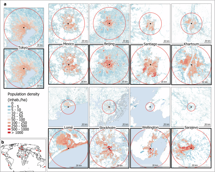
We start by observing how the population density radial (“center-periphery”) structure of cities can be successfully seen through the lens of urban scaling laws. To do so, we use the GHS-POP gridded dataset⁴² (see Methods), and first observe the uneven distribution of population within cities of different sizes through maps. At a similar zoom level, it is very difficult to find consistencies between cities of different sizes (Fig. 1a, thin edge). Indeed, cities have very different population sizes, which makes it challenging to compare their urban structure⁴³. The main reason is that large cities like Tokyo ((Nsimeq 37.4) million inhabitants) are more spread out and tend to be denser than smaller cities like Sarajevo ((Nsimeq 0.3) million inhabitants), as suggested by the above literature. Based on empirical analyses of the average population density (rho (r)) as a function of the distance to the center (r), we find that a rescaling with the power 1/3 of city population ({N}^{1/3}) in each of the three dimensions is appropriate to obtain a homogenous population density across city sizes (see Supplementary Information). Hence, we dilate the Euclidean space through a zoom on the map (r{prime} ={rk}), simultaneously with the vertical dimension of density (rho {prime} =rho k). The dilation factor (k), which allows us to rescale any city of population (N) to the size of Tokyo (the largest city of our sample, taken as a reference without loss of generality), can be expressed as (k={({N}_{{Tokyo}}/N)}^{1/3}). This approach takes off the size effect, leading to more comparable population density patterns across cities (Fig. 1a, thick edge). This implies that as cities grow, they experience two simultaneous phenomena: a densification and an expansion toward the periphery. Even for a city with shape distortions like Wellington, which is surrounded by hills and its harbor, the homothetic transformation remains very effective.

To better capture the radial (“center-periphery”) structure of cities, we derive population density radial profiles from the maps (Fig. 2a), using the average density (rho (r)) as a function of distance (r) from the center. Whatever the size, the population density profile is well-described by a negative exponential function, as straight lines appear on a semi-logarithmic graph. We sometimes observe a “density crater”, which is already well-documented in the literature^8,16, as well as some cities with dense peripheral areas (nearby cities), such as Mexico or Beijing. Despite these peculiarities, curves are well clustered by city size at every distance from the center, indicating that large cities tend to be denser and cover a larger area to accommodate the extra population.

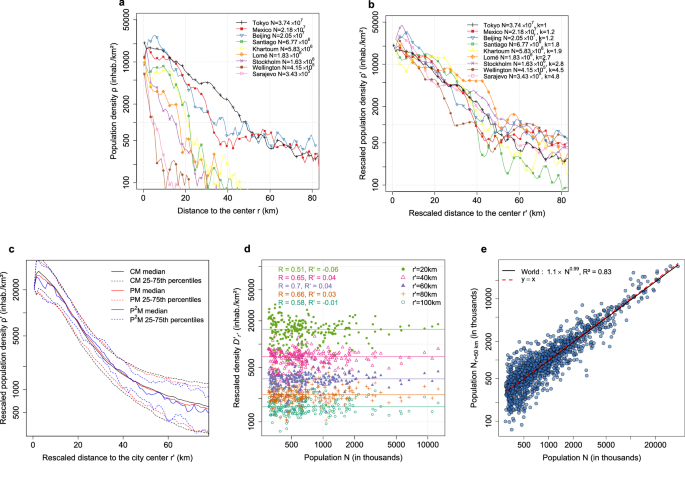
Radial profiles for a sample of nine capital cities displayed both before (a) and after (b) rescaling, on a semi-logarithmic plot. Supplementary Fig. 3 shows the radial profiles for all cities. The population (N) provided by the United Nations (UN) is given in the legend, as well as the rescaling factor (k) (s.t. ({r}^{{prime} }={rk}) and ({rho }^{{prime} }=rho k)). c Distribution of population density rescaled radial profiles ({rho {prime} (r}^{{prime} })) for all cities of the database and under different weighting schemes. d Average rescaled density (D{prime}) in disks of radius (r{prime}) as a function of city size (N). To ensure readability, results are displayed for European cities only (Supplementary Fig. 7 displays the same information for all cities). The correlation coefficient between city size and population density (before and after rescaling, written respectively R and R’) is also given. Note that both variables are presented on logarithmic scales. The horizontal lines represent the median rescaled density ({D{prime} }_{r{prime} }) of cities. e Population within a disc of radius ({r}^{{prime} }=50) km as a function of the UN population. The solid line is a power-law fit (Eq. (1)) with an exponent (0.99pm 0.01).

Following the same approach we used for the maps, we rescale the two Euclidean dimensions of space and the vertical dimension of population density. It allows us to get a view of the intra-urban density structure of cities, for a typical city of the size of Tokyo (Fig. 2b). We notice that our sample of capital cities exhibits similar variations of rescaled density (rho {prime} ({r}^{{prime} })) despite their different history, size, and location on the planet. These regularities indicate that the rescaling with the parameter ({N}^{1/3}) is successful in taking off the size effect and point to a universal structure of cities arising from similar mechanisms. These findings are supported by robustness checks, which suggest that this 1/3 scaling exponent yields the most homogeneous rescaled radial profiles (Supplementary Fig. 2).

To further document the generic radial structure of all cities and the deviations, we compute the median rescaled radial profile and the interquartile range (IQR) with a spacing of 1 km around the center. They show a remarkable concentration of radial profiles around a mean global urban profile (Fig. 2c). To account for the unequal distribution of city sizes^43,44, we also compute those statistics using two additional weighting schemes, the Person Model (PM) and the P² model (P²M), which weight cities with city population and the square of city population, respectively (see Methods). Setting aside the central crater, the density at the center is (rho {prime} left({r}^{{prime} }=0right)simeq mathrm{40,000}) inhab./km² for a theoretical city of the size of Tokyo (Fig. 2c), and drops sharply within the first kilometers from the center. By contrast, our scaling law of population density predicts a density at the center (rho {prime} left(0right)simeq mathrm{27,000}) inhab./km² for a city of 10 million inhabitants, and (rho {prime} left(0right)simeq mathrm{12,500}) inhab./km² for a city of one million inhabitants. These figures represent the first estimate of central density in relation to city population, since this size effect was suggested⁹. We also note that both the median profile and the IQR remain nearly unchanged under the different weighting schemes, denoting that our approach is very robust across the urban hierarchy. This is confirmed by a look at the mean rescaled profiles of different city size classes, which show very small remaining fluctuations (Supplementary Fig. 5b).

These regularities in the radial structure of cities also suggest to look at them through circular disks, instead of rings. This corresponds to integrating (summing) the density from the city center to a given distance, instead of studying the density in a thin ring. For simplicity, we will speak here of rescaled distance (r{prime}) to the center, actually meaning a non-rescaled radius (r={r}^{{prime} }/k) which differs for each city. These disks we define are illustrated for ({r}^{{prime} }=60) km by circles on Fig. 1a. Given a value of the rescaled radius (r{prime}), we define ({N}_{r{prime} }) as the population count, ({A}_{r{prime} }=pi {r}^{{prime} 2}/{k}^{2}) the area, and ({D}_{r{prime} }={N}_{r{prime} }/{A}_{r{prime} }) the density within a disc of rescaled radius (r{prime}) around the city center. The rescaled density is given by ({D{prime} }_{r{prime} }={D}_{r{prime} }times k,) where (k) is the rescaling factor defined above. We test different values of (r{prime}), in order to look at the scaling effect from the urban core (({r}^{{prime} }=20) km) to the whole city (({r}^{{prime} }=100) km). Urban density decreases as (rescaled) distance (r{prime}) from the center increases, because more peripheral areas are encompassed (Fig. 2d). While we find a clear positive correlation between density ({D}_{r{prime} }) and city population (N) ((p)-value < ({10}^{-16})), this correlation vanishes when using the rescaled density ({D{prime} }_{r{prime} }) (see Supplementary Information), indicating that the transformation holds throughout the urban system and along the entire radial profile. This is an important finding for the understanding of urban structures, as it reveals a rather universal shape of cities, which can only be seen if we account for the size effect.

Instead of examining density, we now focus on the fundamental relationship between area ({A}_{N}) and population (N), which is a common question in the urban scaling literature^41,45. This fundamental allometry³⁴ is expressed by the power-law relation

where ({A}_{1}) is a constant corresponding to the theoretical area of a city with one inhabitant, and (gamma) a scaling exponent. However, no city delineation is provided by our UN WUP dataset⁴⁶. Nevertheless, we draw concentric circles of rescaled radius (r{prime}) around the city centers, and look at the relationship between the population ({N}_{r{prime} }) and city size (N). The scaling relationship for ({r}^{{prime} }=50) km returns an exponent (0.99pm 0.01) (R² = 0.83), and the curve is very close to the straight line (x=y) (Fig. 2e). This finding suggests a proportionality and even an identity (on average) between the resident population located in a buffer of radius ({r}^{{prime} }=50) km around the center and the one inside the city boundaries used by the UN. In other words, the city definition of the UN (using many criteria) is roughly equivalent, on average, to a circle of rescaled radius ({r}^{{prime} }=50) km, thus following the homothetic behavior of urban density. Then, if the largest city, Tokyo, can be delineated with a circle buffer of radius (r={r}^{{prime} }=50) km, this distance ({r}^{{prime} }=50) km actually decreases with population, corresponding to (rsimeq 34) km and (rsimeq 10) km for a ten million and a one million inhabitants city, respectively. Since ({A}_{r{prime} }=pi {r}^{{prime} 2}/{k}^{2} sim {N}^{2/3}) as (k sim {N}^{-1/3}), these results regarding population density determine a relationship between area and population of the form (A sim {N}^{2/3}). They also confirm the roughly circular shape of cities, featured in classic models of urban geography^10,47.

Scaling of the parameters

We now aim to describe these radial profiles of population density mathematically with simple statistical tools and a parsimonious approach. To achieve this, we use a limited number of parameters that can be directly interpreted in terms of urban concentration. As suggested by the previous results, we carry out exponential fits for each city. We use a linear fit L of the logarithm (Eq. (2), see Methods), as well as a non-linear fit of the raw value (NL model, Eq. (3)), with two parameters, ({a}_{N}) measuring the density at the center and ({b}_{N}) the characteristic distance (sometimes also referred to as the density gradient). Besides, we try another non-linear (exponential) fit, where we force the relationship ({a}_{N}{b}_{N}^{2}2pi =N) to hold (see Methods), ensuring that the total population in the model corresponds to our UN data. Using the relationship between the two parameters ({a}_{N}) and ({b}_{N}) (Eq. (5), see Methods), this fit is a one-parameter model (1NL model). For comparison purposes, we also fit the profiles using a (negative) power law.

We notice that the exponential function describes empirical data satisfactorily in most world cities, with median R² values of 0.52, 0.95 and 0.91 for the linear, non-linear, and one-parameter non-linear fits, respectively (density plot, Supplementary Fig. 9). These values are high, which suggests that very parsimonious models are able to describe population density profiles. By contrast, the power-law function is clearly outperformed by the exponential (Supplementary Figs. 9–11).

Let us call (alpha) and (beta) the scaling exponents of the fitting parameters ({a}_{N}) and ({b}_{N}) (Eq. (7)). From the 3-dimensional homothetic scaling with the exponent 1/3 observed before, we expect (alpha =beta =1/3). This is rather precisely what we find in Fig. 3, where the expected exponent 1/3 is represented by a horizontal dashed line. For nonlinear models, we note that a weighting scheme that distributes statistical weights more evenly along the urban hierarchy (see Methods), such as the Person and P² models (PM and P²M), brings us closer to these expectations. Conversely, if small cities are weighted as much as megacities (City model CM), we find a higher value for (beta) (horizontal scaling) than for (alpha) (vertical scaling).

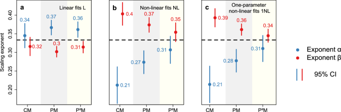
Results of linear fits of the fitted (log) parameters ({a}_{N}) (exponent (alpha)) and ({b}_{N}) (exponent (beta)) against the (log) total population (N). Those parameters ({a}_{N}) and ({b}_{N}) come themselves from the linear fits (a), as well as two-parameters (b) and one-parameter (c) non-linear fits of the radial profiles. We derive these results for three weighting possibilities: the City Model (CM), the Person Model (PM) and the P²M model. The horizontal dashed line represents the expected value (alpha =beta =1/3). The error bars indicate the 95% confidence interval (CI).

We also observe that this scaling behavior is consistent with another theoretical expectation. If cities are circular and population density decreases exponentially with the distance to the center, then the total population can be seen as the volume under the radial profile of density, and a scaling relationship ({a}_{N},{b}_{N}^{2} sim N) holds (see Methods). Hence, the two scaling parameters are connected by the equality (alpha +2beta =1) (Eq. (5)), which aligns with the exponents obtained from the power-law relationships (Fig. 3), in particular, the homothetic scaling (alpha =beta =1/3).

In light of our findings regarding population density, cities of the world are roughly of one shape, exponential cones, which evolve vertically and horizontally with city size. Therefore, the characteristic distance and central density for a city of any size can be expressed as ({b}_{N}={b}_{1}{N}^{1/3}) and ({{a}_{N}={a}_{1}N}^{1/3},) respectively, where we estimate ({b}_{1}simeq 35) m and ({a}_{1}simeq 125) inhab./km² using the results of the 1NL model. Figure 4a provides a theoretical display of the average change in the radial structure of population density, as we move from a small to a large city. Of course, individual cities do not follow precisely these geometric properties, but this lays the foundations for more effective inter-urban comparisons.

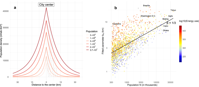
a Illustration of the homothetic behavior of population density radial profiles. The tangent at (x=0) (grey dashed lines) is also shown. b Power-law relationship connecting ({b}_{N}) (from the one-parameter non-linear fit 1NL) and city size (N). The black line gives our expectations, a scaling with the cube root of total population ({N}^{1/3}). The color represents the annual energy use per capita, in kilograms of oil equivalent (in a decimal logarithmic scale).

Indeed, cities have local characteristics likely to infringe on the expected radial structure. The scatter plot presented in Fig. 4b illustrates the relationship between the fitted parameter ({b}_{N}) (from the 1NL model, Fig. 3c) and city size, along with the fluctuations around the scaling law. Although many cities exhibit a center-periphery structure close to the expected homothetic transformation, a closer inspection reveals significant deviations. Some capital cities are rather sprawled, as most of their population is located in peripheral areas (Brasilia, Canberra, Washington D.C), while some other cities are much denser (Dhaka, Cairo). We observe that these different urban forms are linked to the nationwide energy use per capita. Compact cities (with a low value of ({b}_{N}) considering their population) are located in energy-efficient countries, while sprawled cities show the opposite trend. To further investigate regional and national peculiarities, one option is to account for the city-size effect beforehand. Our approach differs in this respect from many studies, which recognize that urban forms vary with city population, but do not account for this effect systematically.

Urban density index

Although our urban scaling framework manages for the city size effect surprisingly well, we still observe significant fluctuations across different locations on the planet (Supplementary Figs. 4–6). Our results suggest a size-independent measure of urban concentration, the urban density index ({rm{UDI}}={b}_{N}/{N}^{1/3}={{(b}_{N}/{a}_{N})}^{1/3}) (see Methods). It corresponds to the residual of the scaling relationship between the parameter ({b}_{N}) and population size (N) (Fig. 4b) and is linked to average density (rho) as (rho sim {{UDI}}^{-2}) (see Methods), so that a dense city will have a low UDI (Fig. 5a). Each population size (N) associates indeed with a range of values for the two parameters ({a}_{N}) and ({b}_{N}), and for the UDI. This index provides a more in-depth comparison between cities by examining how the center-periphery structure of cities deviates from the observed scaling law. It has the dimension of a distance, but could also be considered dimensionless (see Discussion).

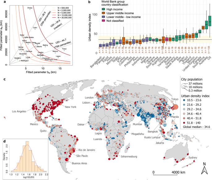
a Relationship between the regression parameters ({a}_{N}) and ({b}_{N}) of the 1NL model and the UDI, for different population sizes. The dots represent the estimated parameters for a selection of capital cities. b Boxplots of the UDI. Results are presented by country and sorted by median value (increasing order, from left to right). The number of cities per country (n) is also given (countries having fewer than 10 cities are not displayed). The color indicates the income group (World Bank). The horizontal line indicates the global median, ({UDI}=34.6), and the colored area the 25^th-75^th percentile range. c Map of the UDI. d Histogram of the logarithm of the UDI. A normal distribution of the same mean 1.5 and standard deviation (sigma =0.19) (red curve) is used as a guide to the eye.

The map and boxplots illustrate the geographical variation in urban concentration measured by the UDI (Fig. 5b, c). It reveals a specific distribution, statistically close to log-normal (Fig. 5d), which mainly seems to oppose developed to developing countries. The latter countries (such as Bangladesh, Egypt, India) have very dense cities, while sprawled cities are mainly located in high-income countries (United States, Australia, Canada). However, there are some exceptions. We note that South African cities have a very flat center-periphery structure, which can be explained by the stringent urban regulations during Apartheid¹⁵. We further observe that there are rather small variations within countries, suggesting similar mechanisms at the national level. Among the global driving forces, wealth measured by income per capita seems to be key, as low-income and lower-middle income countries concentrate compact cities (low value of the UDI), and conversely for high-income countries (Fig. 5b).

We deepen this analysis by exploring how the UDI evolves with a set of indicators obtained at national level (Supplementary Table 2 and Fig. 16). Our results show that two variables are even more closely linked to the UDI than the GDP per capita, namely energy use and number of cars per inhabitant – these are all indicators of the level of development. Indeed, we have ({UDI} sim {varepsilon }^{0.4}) and (rho sim {{UDI}}^{-2}), which gives us (varepsilon sim {rho }^{-1.3}) (Supplementary Information). The interplay between UDI, population density, and energy use per capita can be related to previous work⁴⁸, which finds a negative relationship between average population density (rho) and energy use per capita (varepsilon), and pleads for more compact cities in order to meet the sustainability challenge. Although the question of the most appropriate urban form is still debated in the literature, along with the causal relationship between density and energy use, our results contribute to highlighting that the environmental issues of sprawling, space-consuming cities are clearly linked to the level of development.