Experimental design
Samples
We obtained fresh tissue samples of primary tumors from five patients with uterine cancer (Additional file 1: Table S1), and in three cases, distal “normal” endometrium (see Additional file 2: Table S2 for a detailed description). The tumor types surveyed include two carcinosarcomas, a serous carcinoma, an endometrioid adenocarcinoma, and a leiomyosarcoma. Each sample was frozen and pulverized into a powder. From this powder, nuclei were extracted for single-cell DNA, single-cell RNA, and single-cell DNA-RNA (“hybrid”) BAG platform. We also used the same source material to perform whole-genome sequencing (WGS). This comprehensive approach ensured that all types of cells were proportionately represented in each method of analysis. To refine our methodology and study doublet collisions, we mixed powders from different patients prior to single-nucleus sorting, as discussed later. Additional file 2: Table S2 provides a comprehensive overview of the datasets utilized in our study, detailing the combination of sample origin (including unique setups like the mixed powder experiment), the associated protocols, and the respective experimental parameters.
The hybrid BAG platform
Our study uses the BAG platform, a versatile method that captures templates from a single-cell entity, either whole cells or nuclei. The BAG platform was built for flexibility, allowing for the reagent customization needed to capture DNA and RNA from the same single cells in a high-throughput manner. As described in Fig. 1A–D, nucleic acid templates (or simply “templates”) are captured through primer hybridization to Acrydite-anchored primers embedded into balls of acrylamide gel, shortened to BAGs. This process is followed by primer extension, transcribing the template information of each single cell to primers securely tethered to a single BAG [35]. To establish cell identity, we used a pool-and-split synthesis approach to affix a BAG tag to each template, randomly assigning one of a million identities (963) to every BAG. During pool-and-split, we also introduced a template tag (also known as varietal tag or UMI) to each template. For the hybrid protocol, we used both oligo-TG primers and oligo-T primers to capture DNA and RNA templates, followed by using DNA polymerase and reverse transcriptase to transcribe the templates onto the anchored primers simultaneously. We then prepared sequencing libraries by tagmentation.
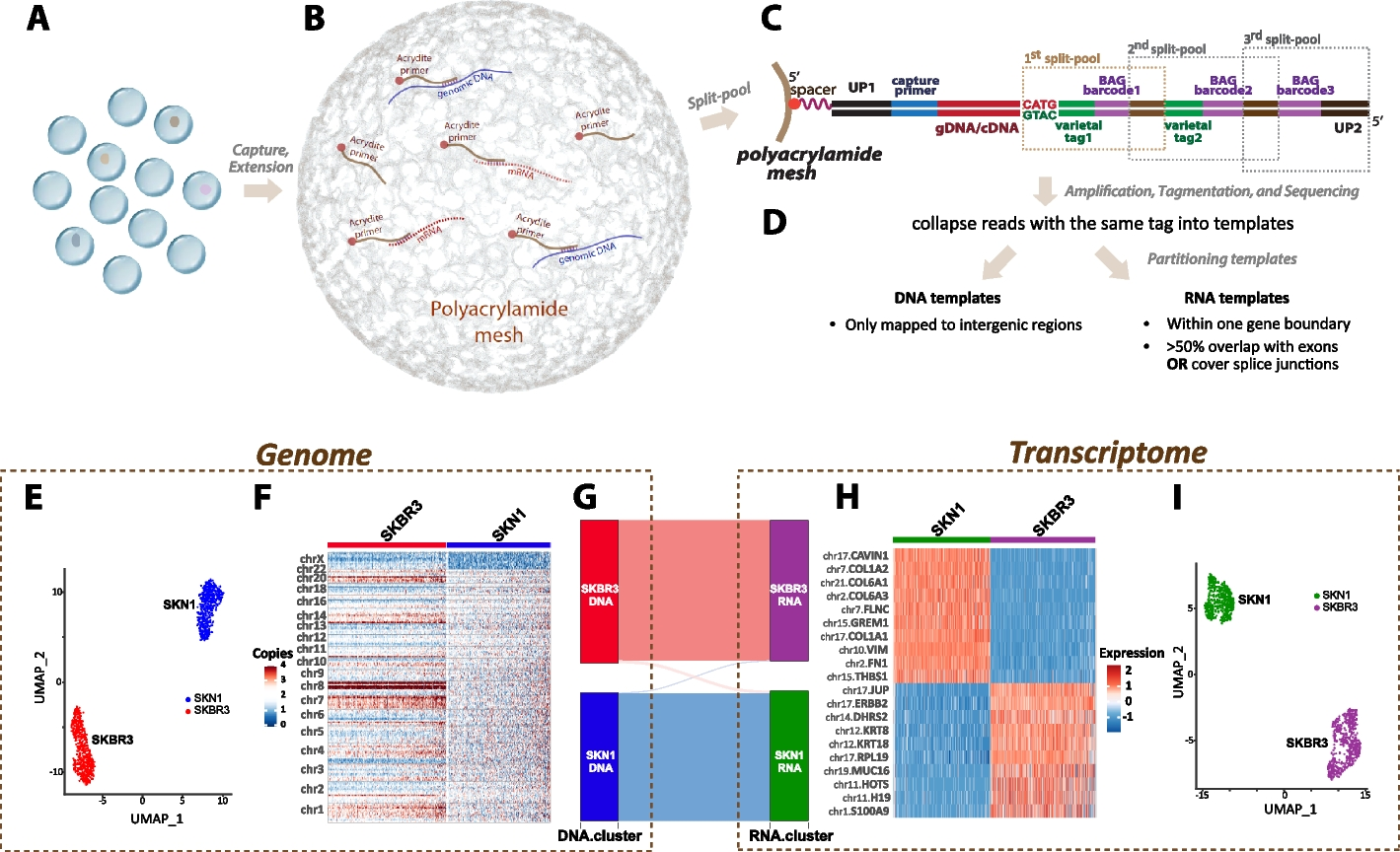
Overview of hybrid BAG-seq protocol and performance on cell-mixture experiment. A–D Key steps for hybrid BAG-seq pipeline. A Encapsulation: Individual cells or nuclei are encapsulated within droplets containing acrylamide and Acrydite-modified primers that are designed to capture both mRNA and genomic DNA. B Polymerization and primer extension: Gel polymerization is followed by primer hybridization. Acrydite primers are extended by reverse transcriptase and DNA polymerase. C Split-and-pool barcoding: The double-stranded cDNA and genomic DNA are cleaved with a restriction enzyme. During successive rounds of pool-and-split, BAG-specific barcodes (purple) and template-specific varietal tags (green) are added. This process uniquely tags each molecule while assigning a distinct BAG barcode to templates in the same droplet. D Sequencing and layer assignment: Post-amplification, the molecules undergo tagmentation and subsequent sequencing. The sequencing reads are analyzed for expected structure, tags are extracted, and reads with identical varietal tags are collapsed into single templates. Templates are then partitioned into either the DNA or RNA layers based on their mapping characteristics. E–I Performance and genome-transcriptome correlation from a SKN1-SBKR3 mixture single-cell hybrid sequencing experiment: E clustering based on DNA copy number; F heatmap of DNA copy number variations across chromosomes for SKN1 and SBKR3 cells; G correlation between genomic clusters and expression clusters; H heatmap of marker genes of expression clusters; and I clustering result based on gene-count matrix
Genomic filters
All three protocols—DNA-only, RNA-only, and hybrid—require mapping reads to the genome and then organizing the mapped reads based on their BAG and template tags. First, each read is checked for having the expected structure of barcodes and primer sequences. Second, with the tag and primer sequences removed, the rest of the read is mapped to the reference genome. Reads that share a template tag and a BAG tag, and that co-localize in the genome, are collected into read aggregates, and operationally considered a captured template. The average number of reads per captured template for each library is also reported in Additional file 2: Table S2.
For classifying molecules into DNA or RNA origin, templates are assigned to either the RNA or DNA molecular layers based on the composition of their read aggregates. As detailed in the Methods section, templates with largely exonic read aggregates are assigned to the RNA layer, whereas templates with strictly intergenic read aggregates are assigned to the DNA layer. Any remaining templates are marked as indeterminate. Based on our observations, we also found it necessary to introduce additional measures to control bias in the hybrid data. First, we observed interference of RNA with DNA clustering. For DNA profiling and clustering, we excluded certain genomic hotspots, mostly poly-T/A-rich regions, to which many nuclear RNA sequences map. This progressively more stringent criterion significantly increased the quality of copy number data from the hybrid protocol, as shown in Additional file 3: Fig. S1. The bin boundaries were determined empirically to achieve uniform template counts using data integrated from the two normal tissues (Normal 1 and Normal 4) in this study. Second, for clustering analyses, we removed BAGs with fewer than 300 RNA-layer molecules or 600 DNA-layer molecules (discarding approximately 20% of all hybrid BAGs, see Additional file 2: Table S2), and then excluded BAGs where the ratio of DNA to RNA templates fell below one-fifth or exceeds five times the average ratio for that library. These BAGs, which constituted only a very small proportion (0–0.5%) of the nuclei passing minimum-count thresholds (Additional file 3: Fig. S2), could represent poor quality in either the RNA or DNA layer and could result in abnormal clustering results if not removed. We applied these categorization rules to all seven tissue nuclei datasets for all three protocols: hybrid, DNA-only, and RNA-only. The full distribution of each category per sample is shown in Additional file 3: Fig. S3A. Using data from one tumor sample as an example, we demonstrated that the layer categorizations are reasonable. Specifically, DNA clustering identities are very similar (97.6% concordance) whether using all molecules or only DNA-layer molecules as bin counts (Additional file 3: Fig. S4) in the DNA-only protocol, and a similar conclusion (95.2% concordance) was observed for gene expression clustering results in the RNA-only protocol (Additional file 3: Fig. S5), when restricting the analysis to the RNA layer or using all of the RNA templates mapped within transcripts.
We initially applied the molecular-layer concept to a mixture experiment involving two human cell lines: a normal fibroblast, SKN1, and a breast cancer cell line, SKBR3. The distributions of the basic parameters and downsampling curves from this experiment are shown in Additional file 3: Fig. S3B–G. We illustrate the clustering results and heatmaps based on the copy number and gene expression in Fig. 1E–I. The genomic and transcriptomic features from the hybrid protocol successfully recapitulate the published features of these two cell lines [35, 42]. The alluvial diagram (Fig. 1G) shows the projection of the genomic clones into the expression clusters. As expected, we observed a good one-to-one correlation between the genome and transcriptome of each cell type. Only 1.06% (10 out of 941) of the cells from the DNA cluster of one cell type (either SKN1 or SKBR3) projected to the RNA cluster of the other cell type, probably due to cell doublets.
Clustering RNA and DNA layers
We used the Seurat package [43] for our single-cell sequencing analysis—a tool widely recognized for its utility in gene expression clustering. For the RNA layer, we followed the standard methodology for expression clustering via “RunUMAP” and “FindClusters” functions. We extended the application of Seurat to cluster the DNA layer. We explored a range of DNA bin sizes and ultimately used a total of 300 bins for the DNA clustering and copy number analysis, as it provided a good balance of genomic resolution and average per-bin counts for a high signal-to-noise ratio and copy number reliability. These empirical bins range from 4.7 to 36.5 Mbp, with a median of 9.5 Mbp, and we treated the normalized raw DNA template count within each bin as a “gene input” for the clustering process and heatmap plotting. The segmentation information was only used for cluster-based copy number profile plotting, as shown in Fig. 2 and Additional file 3: Figs. S6–S9, panel B. This approach allowed us to identify shared copy number profiles that we could leverage in a manner similar to gene expression clustering (further detailed in Methods section).
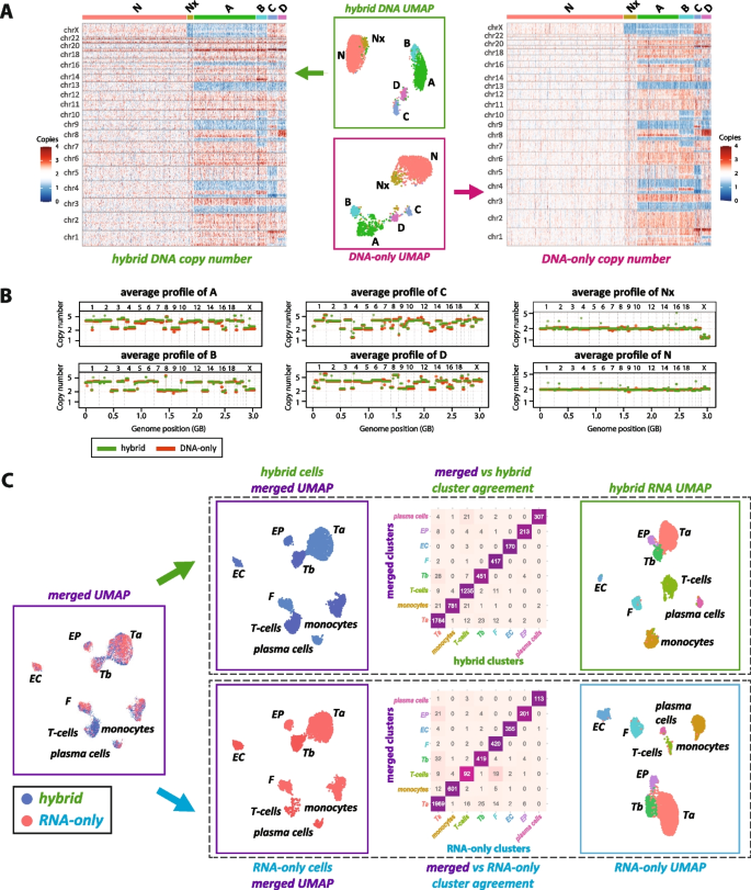
Comparative clustering analysis using the hybrid BAG-seq protocol versus DNA-only and RNA-only protocols. A Single-cell DNA copy number analysis of a tumor sample from patient 2, comparing the hybrid protocol data (green) with the DNA-only protocol data (red). The tumor sample has six distinct copy number profiles: normal diploid cells (N), diploid cells with X chromosome loss (Nx), and four aneuploid tumor clones (A, B, C, and D). Central plots show UMAP visualizations of single nuclei, color-coded according to cluster identity. Adjacent heatmaps display the binned copy number variations for each single nucleus, arranged by cluster identity on the x-axis against genomic bins on the y-axis, with red indicating amplification and blue indicating deletion. B Aggregated copy number profiles derived from summing across all single nuclei within the same cluster, showing high concordance between hybrid (green) and DNA-only (red) datasets. C RNA expression analysis of the hybrid data (green) compared to RNA-only data (blue). To the far left, hybrid and RNA-only data are co-clustered into eight expression clusters: two tumor expression clusters (Ta and Tb) and six somatic cell types—fibroblasts (F), epithelial cells (EP), endothelial cells (EC), T-cells, monocytes, and plasma cells. These merged clusters are then segregated by hybrid or RNA-only origin. To the far right, each protocol’s data are independently clustered into the same eight expression clusters. The central heatmaps quantify the agreement between the merged clusters with the respective hybrid and RNA-only clusters. Analogous plots for the other four patients are presented in the supplementary figures
Multinomial wheel
Whether dealing with DNA or RNA data, a common question often arises: how well does a single cell “fit” within its assigned cluster? To investigate this question within the context of a pre-established set of clusters, we first use multinomial probabilities. We take as a given the N clusters that Seurat identifies. For each cluster, we sum the gene (or genomic bin) count data over the cells in that cluster and normalize by the total template count. This results in a probability vector that represents the average gene frequency of the cluster. Utilizing this vector, we can calculate the probability that an observed single-cell count vector arose from each of the N clusters.
However, multinomial probabilities do not translate into a useful metric for deviation from a cluster. Every cell is assigned with almost no ambiguity to one of the major clusters. To properly identify cells that fall between clusters, we incorporate mixed cluster states into a multinomial wheel. For every pair of clusters, A and B with multinomial vectors pA and pB, we also consider the mixed state ABα with multinomial vector α pA + (1 − α) pB for α in [0.1, 0.2, …, 0.9]. This results in a total of 9*(N choose 2) + N cluster states. By doing this, we can segregate the cells into two categories: core cluster members that stay close to an original cluster, and transitional members that fall between two clusters.
The hybrid platform is comparable to DNA-only and RNA-only platforms
In this section, we compare the hybrid BAGs to the DNA-only and RNA-only BAG platforms. We first focus on comparing the hybrid DNA layer to the DNA-only data, and then the hybrid RNA layer to the RNA-only data. We use the tumor tissue sample from patient 2 as a representative example, with similar comparisons for the other tumor tissue samples provided in Additional file 3: Figs. S6–S9.
DNA layer
Figure 2A compares the DNA layer from the hybrid data (left) with the data from the DNA-only BAG protocol (right). The central scatter plots display the clustering results in UMAP space, with the hybrid data (in the green box) above and the DNA-only data (in the red box) below. Each point represents a single nucleus, color-coded by its DNA copy number cluster. Both methods resolved six clusters, which we manually aligned based on pattern similarity. The N cluster includes cells with a typical diploid profile, whereas the Nx cluster represents a subpopulation of diploid cells with loss of an X chromosome. The remaining clusters—A, B, C, and D—exhibit varied aneuploid copy number profiles. The adjacent heatmaps illustrate the distribution of copy number changes across the genome, with deletions in blue, amplifications in red, and the diploid state in white. Each single cell is represented by a column and the cells are grouped by their DNA cluster.
To verify the congruence of profiles between platforms, we compared the average copy number profiles for each cluster in Fig. 2B, with DNA-only data in red and the DNA layer of the hybrid data in green. To quantify the similarity of clustering results between the two protocols, we used the multinomial wheel approach to measure the proximity of every single tumor nucleus to the centroids of tumor clones determined both by its own protocol (either hybrid or DNA-only) and by the other protocol. As shown in Additional file 3: Fig. S10, projecting DNA-only data to either DNA-only multinomial states or hybrid multinomial states showed no signal reduction (84.5% versus 84.5% nuclei within 2 units to the centroids), and similarly high concordance was observed when projecting hybrid data to either hybrid multinomial states or DNA-only multinomial states (77.2% versus 68.9% nuclei within 2 units to the centroids). Additionally, we examined heterozygous SNPs in both platforms and found similar patterns of loss of heterozygosity (LoH) and allele imbalance. These allele imbalance patterns (Additional file 3: Fig. S11) align with the copy number calls, in that when the copy number is an odd integer, allele imbalance is always observed.
RNA layer
We next analyzed the RNA layer of hybrid data compared to the RNA-only protocol. We first combined all the nuclei from both the hybrid and RNA-only platforms and clustered the integrated dataset into 8 clusters as shown in Fig. 2C (leftmost “merged UMAP” plot). While each cluster is labeled with a unique identifier, hybrid nuclei are shown in blue, and RNA-only nuclei in red. We then split the merged dataset by experimental origin with hybrid nuclei shown above and RNA-only nuclei below. The rightmost plots in the panel reflect the clustering of each dataset independently into the same eight identified categories.
We reserve a discussion of the differentially expressed genes for later, but currently label the clusters as monocytes, T-cells, F (fibroblasts), EC (endothelial), EP (epithelial), plasma cells, and two distinct tumor RNA clusters, Ta and Tb. The central agreement matrices, formatted as heatmaps, show the consistency of cell classification across platforms within the merged dataset. The top matrix compares hybrid cluster assignments to merged dataset classifications, while the bottom does the same for RNA-only data. For both datasets, a significant proportion (95%) of cells align diagonally, confirming that cluster identities are well preserved across the two platforms.
Profiling genome and transcriptome of tumor samples using hybrid data
For each of the five tumors, we clustered the DNA and RNA layers of the hybrid data, respectively (Fig. 3). The DNA clusters are presented on the far left, accompanied by copy number heatmaps similar to the previous illustrations. On the far right, RNA clusters are displayed, along with a heatmap that illustrates the relative expression levels across sets of differentially expressed genes (blue for low expression, red for high).
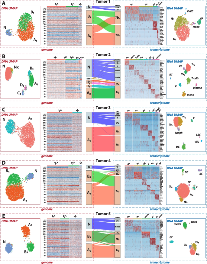
Connecting genomic and transcriptomic data across five tumor samples using alluvial diagrams. A–E Summary of the hybrid data analysis of tumor tissue samples from five individual patients, show the various connections between genomic and transcriptomic landscapes. For each patient: The “genome” sections on the left, bordered in red, display the DNA layer information, including UMAP visualizations of single nuclei colored by genomic cluster identities and accompanying heatmaps showing copy number variations across the genome. The “transcriptome” sections, bordered in blue, present the RNA layer data, including UMAP plots of single nuclei colored by expression cluster identities. These are accompanied by heatmaps of marker genes that are distinctly upregulated within specific expression clusters. At the center of each panel, alluvial diagrams connect the DNA and RNA data, linking genomic cluster identities (left) to the RNA expression clusters (right). The thickness of the flow lines represents the proportion of nuclei that belong to a specific genomic cluster (X) and an expression cluster (Y), illustrating the integrative analysis facilitated by the hybrid BAG-seq platform
Based on the dual DNA and RNA identities assigned to single cells in the hybrid dataset, we quantified the frequency with which cells from a specific DNA cluster appear in a given RNA cluster. This cross-layer association is visualized using alluvial diagrams. For example, in panel A from Tumor Sample 1, the alluvial diagram illustrates that the diploid N cells map exclusively with non-malignant expression profiles (macrophage, F + EC, and EP). Conversely, both tumor clones A1 and B1 map to the two tumor expression profiles (Ta1 and Tb1).
We now delve into the unique characteristics of each of the five tumor specimens, drawing comprehensive insights from both DNA and RNA layers. Focusing on the tumor genome projection patterns, each of the five tumors displayed a different projection pattern, and we observed almost all the possible patterns. To classify projections, we used a set of letters and numbers to represent the tumor genome and tumor RNA clusters, respectively. For example, [A:1,2; B:2] indicates tumor clone A projected into RNA clusters 1 and 2, whereas tumor clone B from the same primary tumor tissue projected only into RNA cluster 2. We have seen: distinct tumor clones could each project into distinct expression clusters (e.g., [A:1; B:2] for Tumor 5), into shared clusters (e.g., [A:1,2; B:1,2] for Tumor 1), or into a combination of distinct and shared clusters (e.g., [A:1,2; B:1] for Tumor 4). Alternatively, multiple DNA clones could project into a single RNA cluster (e.g., [A:1; B:1; C:2; D:2] for Tumor 2), or a single tumor clone could project into two RNA clusters (e.g., [A:1,2] for Tumor 3). Furthermore, based on the alluvial plots and the underlying tumor cell identity contingency tables, we calculated the Rand Index and Adjusted Rand Index to quantify the correspondence between DNA and RNA cluster assignments (Additional file 4: Table S3). Higher values of these indices indicate stronger concordance between the two clustering schemes. Tumors 2 and 5, which showed more evident alignment between DNA and RNA clusters, exhibited higher Rand Index and Adjusted Rand Index values compared to Tumors 1, 3, and 4. The latter tumors displayed more mixed projections across modalities, suggesting greater transcriptional plasticity.
With the details of the five cases using the hybrid protocol provided in Additional file 5: Supplementary text, we briefly highlight the important findings regarding these respective cases here.
Tumor 1 was a uterine carcinosarcoma, which is pathologically observed as a biphasic tumor containing both carcinomatous and sarcomatous components. Echoing this in the RNA analyses, cluster Ta1 showed high expression of fibroblast-specific genes, including FGFR3, COL9A2, and COL27A1, in keeping with the pathological classification of this tumor as having a sarcomatous component, whereas these fibroblast genes had lower expression in cluster Tb1. This separation between Ta1 and Tb1 in gene expression patterns was consistent across the hybrid, RNA-only BAG protocol, and 10 × Chromium v3 platform (Additional file 3: Fig. S12). We found that the two tumor clones, which mainly differ in copy number of chromosome 13, each project equally to tumor RNA clusters Ta1 and Tb1. To explore whether any hidden patterns were missed during clustering, we projected DNA-layer clone identities onto the RNA-layer UMAP space and found that nuclei from both DNA clones are randomly interspersed, showing little correspondence between DNA and RNA clusters (Additional file 3: Fig. S13). Similarly, randomly interspersed patterns were observed when projecting RNA-layer cluster identities onto the DNA-layer UMAP coordinates. Tumor 2 is a uterine serous carcinoma and presents a more complex DNA and RNA landscape than Tumor 1. The tumor sample served as our example in the previous section comparing the BAG platforms (Fig. 2). In contrast to Tumor 1, the DNA-RNA correspondence in Tumor 2 is visually more straightforward: tumor DNA clones A2 and B2 mainly project to RNA cluster Ta2, while clones C2 and D2 correspond to Tb2. Regarding resolution of the RNA-layer clustering of the hybrid protocol, we stopped at the hierarchical level where both the hybrid and RNA-only protocol yielded consistent clustering patterns and featured genes. We did not pursue finer subdivisions of RNA clusters that appeared in only one protocol. Given the hierarchical nature of RNA clustering, we report the top-level, biologically meaningful RNA clusters for correspondence analyses and alluvial plots. This rule applies to all five cases. However, in cases where distinct DNA clones are associated with a shared RNA expression profile, such as A2 and B2 with Ta2, we further dissect the RNA cluster to test whether these DNA subgroups differ in gene expression. To assess how copy number variation affects gene expression, we compared gene expression profiles between the subgroups Ta2-A2 and Ta2-B2, as well as Tb2-C2 versus Tb2-D2, as shown in Additional file 3: Fig. S14. The top genes separating these subgroups are not necessarily located in regions with copy number differences that distinguish the two DNA clones.
Tumor 3 is an endometrial adenocarcinoma. It contains a single tumor DNA clone that projects to two distinct RNA clusters—one estrogen receptor (ER) positive and the other ER negative. This observation is consistent with the pathological findings, with the immunohistochemistry (IHC) images showing that ER-positive and ER-negative tumor cells are spatially intermixed within the tissue (Additional file 3: Fig. S15).
Tumor 4 is another uterine carcinosarcoma case. Unlike the other carcinosarcoma case Tumor 1, the tumor cells here globally exhibit sarcomatous-like features, with one RNA cluster, Ta4, comprising about 90% of the tumor cells. These cells are proportionally derived from two distinct tumor DNA clones, A4 and B4, which show substantial differences in copy number. In contrast to this major cluster, a smaller tumor cluster, Tb4, exhibits upregulation of genes related to cytoskeletal organization, cell motility, protein synthesis, and cellular metabolism, and is primarily derived from clone A4. In addition, unlike the first three cases, a separate RNA cluster characterized by proliferation markers is clearly distinguishable at this clustering resolution, but disproportionately comes from one tumor DNA clone A4. As in previous cases, when multiple DNA clones project to a single RNA cluster, we performed differential expression analysis between the DNA-defined subgroups, in this case, Ta4-A4 and Ta4-B4. While there are significantly differentially expressed genes between these two subgroups (Additional file 3: Fig. S16A), the projections of A4 and B4 onto Ta4 appear randomly intermixed in the RNA UMAP space (Additional file 3: Fig. S16B), similar to what was observed in the tumor RNA clusters of Tumor 1. This suggests limited correspondence between DNA copy number variation and RNA expression, despite the much more pronounced genomic differences between clones A4 and B4 compared to the differences between A1 and B1.
Tumor 5 is a uterine leiomyosarcoma, with the most intuitively straightforward tumor DNA-RNA correspondence among these five cases, as it exhibits a nearly one-to-one mapping between the two tumor DNA clones and two RNA clusters, despite some cross-projections. Similar to Tumor 4, an RNA cluster representing proliferating cells is distinguishable at this hierarchical level, but unlike Tumor 4, both tumor DNA clones proportionally contribute to this cluster Tc.
Combined clustering of all patient samples
Integrative clustering analysis and cluster phylogeny
In our previous sections, we examined one patient at a time, while in this section, we aim to understand how patient expression profiles interrelate and potentially achieve finer resolution in our clustering analysis. To gain such a global picture of the hybrid data, we performed cluster analysis on the combined data from all patients, separately for RNA layer and DNA layer, as demonstrated in Fig. 4. For RNA layer clustering, we lowered the threshold for RNA template count from 400 to 300. This analysis includes hybrid data from the five tumors (Tumor i) presented in the previous section, as well as normal tissue samples from patients 1, 2, and 4 (Normal i). We then explore which expression clusters map to which patient and within each patient to which genome cluster, diploid copy number (flat), diploid copy number with one chromosome X (X-loss), or complex aneuploid genome (CN +). In this way, we reveal diverse and common cellular and functional repertoires. These results are summarized in Table 1.
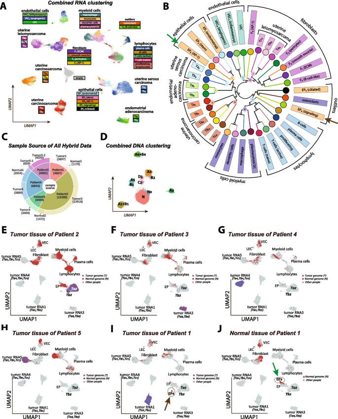
Integrated cluster analysis and unique cluster identification using aggregate tumor and normal tissue data from all patients. A UMAP scatter plot showing the RNA layer data from both tumor and normal tissue samples across all patients, totaling 40,149 nuclei. Stromal clusters are defined through iterative subclustering, while tumor subclusters are defined from individual tumor analyses as presented in Fig. 3. An empty cluster (gray) consists of nuclei mainly from the RNA layer of seven DNA-only experiments. Each point is colored according to the cluster with the highest likelihood as determined by a multinomial model. B The neighbor-joining tree illustrates the relationships among the stromal and tumor subtypes. The tree is computed from inter-cluster distances based on multinomial distributions. C The source of nuclei from the hybrid protocol used in the combined analyses. D Combined DNA clustering after removing nuclei clustered to the “empty” state of the RNA clustering in A. E–J The tumor-genome (blue) and normal-genome (red) nuclei projections on the RNA UMAP space for six tissue samples. The tumor-genome or normal-genome information is determined by the combined DNA analysis in C. Unique stromal components specific to certain tissues are circled in dashed lines and indicated by arrows in I and J, and marked in B
Specifically, our gene expression clustering procedure incorporates several novel features, which we detail below for clarity. First, we include 3500 “empty” cells derived from the RNA layer of DNA-only BAGs. These empty cells were clustered together in Fig. 4A. This cluster also attracts hybrid BAGs with severe RNA template depletion. Overall, 2.4% of hybrid cells coalesce into the empty state.
As before, we use Seurat’s FindClusters and UMAP functions to cluster and display 40,149 nuclei, which uses the UMAP coordinates to visualize the single cells, as shown in Fig. 4A. After the initial clustering, we further resolved the diploid cells to delineate subpopulations, described in the next section. Specifically, we chose four sub-regions of the initial UMAP (blood elements, fibroblasts, endothelial cells, epithelial cells) for further subclustering. Given the single-cell pool’s diverse cell type composition—ranging from tumor, epithelial, endothelial, myeloid, etc. —an iterative clustering approach is a reasonable strategy. For the tumor subclusters, we adopted the case-specific cluster information defined in the previous section.
We use UMAP coordinates to obtain a planar representation of the cells, and our method of multinomial analysis to color the cells by expression type. The aggregate of templates in each subcluster forms a gene probability vector, wherein the total number of templates mapping to a gene is normalized by the total number of templates mapping to any gene, resulting in a probability distribution. This probability vector determines a multinomial distribution for each cluster that in turn, assigns a cluster probability for each single cell based on its gene counts. In Fig. 4A, each point’s color reflects the cluster most likely to have generated the gene counts in that cell.
We then use the multinomial distributions to establish a distance metric between any two subclusters, each with its own multinomial distribution. The asymmetric disparity between two multinomial distributions, A and B, is determined by simulation, in which we determine the number of unique RNA-layer templates of a cell simulated from distribution A that are needed to preferentially assign the cell to A rather than to B, for some given confidence threshold. We then symmetrize the disparity measure, combining A to B and B to A. Clusters with distinct profiles will require fewer templates to establish separation, while those with similar profiles require more templates for differentiation. We invert this measure to establish a pairwise distance (Additional file 3: Fig. S17) and use neighbor-joining to build a phylogeny over the expression clusters (Fig. 4B). We rank the genes that best separate two sets of expression clusters, A and B, using binomial methods, rather than the FindMarkers function within Seurat. We use the ratio of total templates in A and B to determine the null expectation of the ratio for any given gene. We then apply a binomial test to the observed counts for each gene in A and B. The marker genes distinguishing tumor expressional subclusters for each patient can be found in Additional file 6: Table S4, while those for stroma clusters across all five patients are listed in Additional file 7: Table S5.
On the DNA front, from a total of 35,369 nuclei from the sources indicated in Fig. 4C studied using the hybrid protocol, after removing the 2.4% (859 out of 35,369) low-quality nuclei that were clustered into the empty state in the gene expression clustering result, we clustered the DNA-layer of all the remaining nuclei based on genomic bin counts. Similar to the RNA clustering result, in the DNA space in Fig. 4D, tumor-genome clusters were quite distinct from the normal-genome clusters, and distinct clones within a patient mapped nearby to each other or merged into a single cluster at this resolution of clustering.
Common and unique features in stromal subpopulations
Combining RNA and DNA clustering information, the projections of nuclei from six sample sources into the combined RNA space (Fig. 4A) are shown in Fig. 4E–J, where nuclei from a given sample are highlighted either in blue or red, depending on whether they are classified by DNA as tumor or normal genomes. In each panel, the nuclei from other samples are colored in light gray. The projections of the tumor genomes are very distinct between patients, well separated from each other and the projections of the normal genomes.
Although the normal-genome stromal clusters are mostly shared between patients, the distribution and abundance of different subtypes vary significantly by patient and sample. For example, there are substantial differences in immune cell proportions among the five patients, as illustrated in Fig. 4E–J with more quantitative data in Table 1, suggesting variation in tumor microenvironment and immune response. In addition, there are several gene expression clusters that only belong to certain tissues and certain patients, implying influences from tumor microenvironments and personal genomes. For example, the epithelial-like cluster EP4 (Fig. 4I, indicated by the brown arrow) from the tumor tissue of patient 1 is significantly different from the EP3 cluster (Fig. 4J, indicated by the green arrow) from the distal normal uterine site in the same patient, and they are both distinct from the main epithelial cluster EP1. These two clusters are also pointed to by arrows in the hierarchical wheel in Fig. 4B, far away from each other. We believe these distinct clusters are not due to batch effects or template counts, not only because they have distinct and biologically plausible gene expression patterns (Additional file 7: Table S5), but also because these distinct clusters overlapped well in experimental replicates and showed the same patterns in RNA-only datasets (Additional file 2: Table S2). These unique stromal subpopulations will be discussed in detail in the following section.
From a hierarchical and phylogenetic perspective, the multinomial tree (Fig. 4B) provides a more quantitative view of these diverse stromal and tumor RNA clusters. The branches of the tree largely preserve cell-type categories. The blood elements share a common branch (blue labels) with a myeloid-derived sub-branch (dark blue) distinct from lymphocytes (light blue); a branch of epithelial cells (orange); fibroblasts (purple) and endothelial cells (green). Most of the subclusters fall on their expected branch. The exception includes a single sub-branch containing two epithelial subclusters, EP4 and EP5, and osteoclasts, a myeloid cell type. In general, clusters that are close together in the UMAP (Fig. 4A) share a common branch in the tree (Fig. 4B). The major exception is cluster F5, B-cell-like fibroblasts, which are near the B-cells in the UMAP but nearer to the fibroblasts in the tree.
The tumor clones from each patient occupy distinct sub-branches in the tree. The uterine leiomyosarcoma (purple), a muscle-derived tumor, has expression subclusters on the fibroblast branch of the tree. The other four tumors share a deep branch with the epithelial cells. One sub-branch contains the two uterine carcinosarcomas (red and dark red). Nearer the epithelial cells in the tree, are the endometrial adenocarcinoma (green) and nearer still the uterine serous carcinoma (blue). The branch lengths provide a relative measure of similarity, showing that Ta1 and Tb1 are highly similar as are Ta3 and Tb3. In contrast, the subclones of Ta2 and Tb2 are far apart.
Multinomial wheel and crossovers
In the previous section, we observed that the majority of nuclei exhibit concordant DNA and RNA profiles: diploid DNA with stromal RNA expression (flat, N) or complex DNA patterns with tumor RNA expression (CN +, T). These concordant nuclei constitute the expected biological behavior; however, there are a subset of cells that do not match this pattern. Additional file 8: Table S6 shows the counts for each patient of cells that are diploid or complex (flat or CN +) and map to normal clusters or tumor clusters (N or T). Across all patients and tissue samples, 1–5% of nuclei have flat copy number profiles and tumor expression patterns, or a combination of copy number variations and stromal expression patterns. Although accounting for a small proportion of the total dataset, these crossover nuclei may represent an interesting population. Alternatively, they may be the result of unresolved doublet collisions [44]. Additional file 9: Table S7 summarizes the counts and calculates the proportion of concordant and crossover nuclei per patient.
To determine if crossover nuclei are a unique biological state or collision artifacts, we employed the multinomial wheel to differentiate mixed states. Integrating DNA-layer data across all hybrid-protocol experiments, we constructed a multinomial wheel with tumor clusters, diploid cells and diploid cells with X-loss as the individual spokes of the wheel (Additional file 3: Fig. S18A). Some tumor DNA clusters are so similar (A1 and B1, A4 and B4) that we collapse each of those pairs into a single node (A1/B1 and A4/B4). For each pair of the 11 vertices, we created 9 equally spaced sampling states, resulting in a multinomial wheel with (11 choose 2) = 55 spokes and 9*(11 choose 2) = 495 intermediate states.
From the DNA counts of each nucleus, we evaluate the probability that those observations are derived from each of the (495 + 11) = 506 multinomial distributions in the wheel. We assign each nucleus to the node with the highest posterior probability. Notably, more than 60% of nuclei align with a “pure” cluster on the multinomial wheel by residing on a vertex, and 85% are situated within two units’ distance from a pure cluster (Additional file 3: Fig. S18A). Informed by two mixture experiments, detailed in the Methods and Additional file 3: Fig. S18B–E, we apply a collision filter, marking for removal nuclei that are 3 or more units from a vertex and fall between a normal DNA cluster (N, Nx) and a tumor DNA cluster (Ai, Bi, etc.). Additional file 7: Table S5 and Additional file 8: Table S6 (filtered nuclei) show the counts after applying the collision filter.
If crossovers are the result of cryptic collisions, the collision filter will disproportionately reduce the frequency of crossovers compared to the concordant nuclei between the DNA and RNA layers. Indeed, our observations align with these expectations: while the collision filter removed 14% of concordant nuclei, it removed a substantial 71% of crossover nuclei (Additional file 8: Table S6). Removing collisions does not alter the results presented in the previous section. A version of Table 1 restricted to nuclei that pass the collision filter can be found in Additional file 10: Table S8.
The multinomial wheel can be used for much more than detecting doublets. It quantitatively measures how much a single cell deviates from the centroids of major clusters in DNA or RNA space and can provide insights into genomic heterogeneity, particularly for cells transitioning between states. It does not rely on PCA or UMAP coordinates, and by using only cluster centroids as reference points, it offers an interpretable, coordinate-free metric for cell-wise distance that aids interpretation of nonlinear, reduced-dimensional embeddings such as UMAP. For example, in Additional file 3: Fig. S19, we extracted tumor cells from three cases in which only two major tumor clones were present and projected them onto a one-dimensional space based on their best multinomial probability. The proportion of cells classified as “in transition” by the one-dimensional multinomial wheel agrees with the intuitive spatial distribution observed in UMAP space and is significantly higher than expected from doublet rates, suggesting the presence of intermediate or transitioning cells that share features of both clones.
Loss of X chromosome in stromal lineage
In this final analysis, we revisit the occurrence of X chromosome loss in diploid cells, particularly noted in the plasma cell population from patient 2’s tumor sample. X chromosome loss, while reported before in various tissues associated with cancer [45, 46] or aging [47, 48], presented an unusual prevalence in our dataset among the stromal cell types in the tissue. For example, about half of the plasma cells in patient 2 exhibited X chromosome loss, a finding that merited further investigation into its biological implications.
To determine whether the X chromosome loss was the result of a clonal event or occurred independently across different cells, we performed a haplotype analysis: If all affected cells lost the same X chromosome, it would suggest a common ancestry; whereas if they lost different copies of the X, it would point to independent, convergent events. The tumor genome from patient 2 has two subclones with X-loss (A2, B2), and we used these two subclones to phase the SNPs on the X chromosome. Upon aggregating SNPs within each nucleus, we found that the Plasma-Nx nuclei share a common haplotype, suggesting a clonal nature, whereas the T-cell-Nx population shows both haplotypes (Fig. 5A). Given the robust coverage of the Plasma-N and Plasma-Nx subclusters, we were able to conduct a differential analysis on their aggregate gene expression data. As shown in Fig. 5B, there are four genes with significantly different expressions: XIST and TSIX are under-expressed in the X-loss population, affirming the X-loss observed in the DNA layer. The other two genes are IGHG1 and IGHG2, hinting at a potential compositional difference between these plasma cell populations. As XIST RNA is required for X chromosome inactivation and is only expressed from the inactive X chromosome [49,50,51], these results also verify that nuclei from the “Nx” DNA clone lost their inactivated X chromosomes.
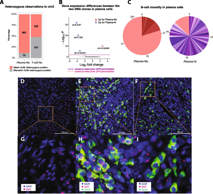
Analysis of chromosome X loss in somatic cells of the primary tumor 2. A Bar plot showing the ratio of X-haplotype observations in the X-loss populations of plasma (Plasma-Nx) and T-cell (T-cell-Nx) nuclei from patient 2. Tumor subclones A2 and B2 with only one copy of the chromosome X are used to phase the X chromosome SNPs in the Plasma-Nx and T-cell-Nx populations as belonging to one haplotype (red, match A2/B2) or the other (gray, mismatch A2/B2). T-cell-Nx nuclei exhibit a balanced distribution of SNVs from both haplotypes, while Plasma-Nx nuclei show a pronounced bias toward the A2/B2 haplotype. B A volcano plot shows the genes with statistically significant expression differences between diploid plasma cells (Plasma-N) and plasma cells with one X chromosome (Plasma-Nx). C Pie charts showing VDJ recombination results for Plasma-N and Plasma-Nx nuclei. Each color represents a unique B-cell clone identified by its CDR3 sequence, with the size indicating the clone’s prevalence. The Plasma-N chart shows a diverse clonal makeup with few dominant clones, while the Plasma-Nx chart shows a clear dominance of one lineage (red), constituting 80% of the population and matching the signature of the primary clone in Plasma-N. D–I Spatial transcriptomics images illustrating XIST expression in the same tumor tissue of patient 2. D RNAscope images displaying the expression of XIST (red) along with DAPI staining of nuclei, showing half of the cells with no XIST signal detection. E, F IGHG (green, plasma cell marker) and XIST (red) expression along with DAPI staining of nuclei. E shows a region consisting of normal plasma cells with XIST gene expression, while F shows another region of plasma cells with no XIST red dots detected. G–I are zoomed-in images of D–F, respectively
Considering the distinct IGH expression in the plasma subclusters, we further investigated the clonality of the Plasma-Nx population through VDJ recombination analysis. Using MiXCR [52] to count the unique VDJ recombination patterns, our analysis strongly suggests that the Plasma-Nx cells are primarily derived from a singular B-cell lineage expansion, in contrast to the Plasma-N cells, which originated from a diverse array of lineages (Fig. 5C).
To corroborate our findings and further visualize the loss of the X chromosome, we applied RNAScope technology on the same tumor tissue from patient 2. The spatial transcriptomics images (Fig. 5D–I) provide a vivid illustration of the XIST expression patterns. DAPI staining (blue) marks the nuclei, while XIST (red) and IGHG (green) show specific gene expressions. In Fig. 5D, half of the cells display no XIST signal, indicating X-loss, likely from tumor A2 or B2 clones with deletions in the X chromosome. Figure 5E and F show IGHG, the plasma cell marker, and XIST expression within two different regions, showing two opposite phenomena. While most of the plasma cells in Fig. 5E contain the XIST signal, implying the presence of the inactivated X chromosome; the majority of the plasma cells in Fig. 5F lack the XIST signal, suggesting that these cells have lost the inactivated X chromosome. Both the plasma cells with and without XIST signals were found spatially localized in the tumor microenvironment.
We next extended our X-loss analysis to the other tissue samples. For patient 1, we noted a 5% X-loss in the diploid component of the normal distal sample, predominantly in the smooth muscle (F2) expression cluster. However, establishing clonality in this context was challenging because the tumor subclones in this patient retained both X chromosomes, making it difficult to phase the lost X haplotype for validation. In patient 4, we identified significant X chromosome loss in the blood component of the normal distal sample, particularly in naïve and active T-cell populations. Additionally, a smaller but notable percentage of fibroblast ECM and smooth muscle cells (F1 and F2) also exhibited X-loss. In contrast, patients 3 and 5 displayed minimal X chromosome loss, accounting for 0.5% of the diploid population.