TrueSpot: a robust automated tool for quantifying signal puncta in fluorescent imaging | Genome Biology

TrueSpot uses an automated threshold selection algorithm that utilizes multiple approaches

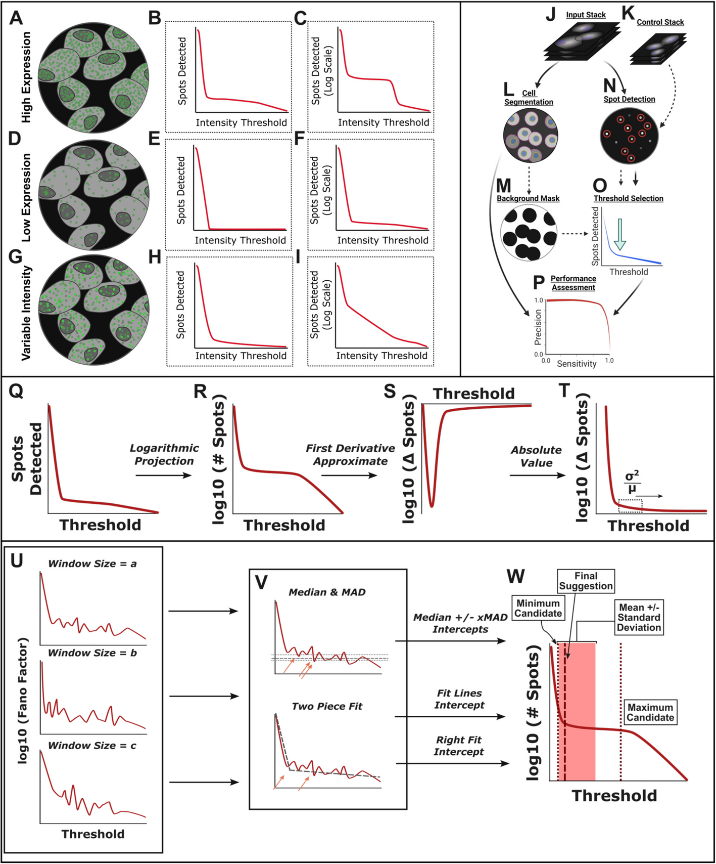
TrueSpot accepts either a 2D image or 3D image stack (which may or may not include multiplexed channels) as input along with an optional control image (Fig. 1J,K). The sample and control are then passed through the initial spot detection module (Fig. 1N). Here, a Laplacian of Gaussian (LoG) filter [6, 7] is applied to the image and coordinates of local intensity maxima in the filtered image are recorded. A range of threshold values is scanned to determine which identified maxima are dropped at each tested threshold. The number of spots/maxima retained at each threshold in the sample image is then plotted against the threshold value as the first step in automatic threshold selection (Fig. 1O). If a control image is not provided, a background mask can be derived from a cell segmentation mask (our cell segmentation module is discussed in a previous publication [23]) and the masked image can be used as a control instead (Fig. 1L,M). The use of controls is entirely optional—their purpose is to assist the threshold selector by finding a noise ceiling. This functionality is however not required to elicit high performance from the threshold selection algorithm, as it was not utilized in any of our simulated image tests, nor in many of the experimental image groups (Fig. 3).

Performance is assessed using recall (also called “sensitivity”) (Eq. 1A) and precision (Eq. 1B) as benchmarking measures across all thresholds, at the selected threshold, and in single cells (Fig. 1P). Area under the precision-recall curve (PR-AUC) was used to evaluate overall detection performance across all tested thresholds. The maximum recall (highest value for recall reached for a tool on a given image across all tested thresholds) was used to distinguish between relative precision and recall contributions to PR-AUC. We used the F-Score (Eq. 1C), a quantification of the trade-off between precision and recall, at auto-selected threshold values to assess tools’ ability to automatically select appropriate thresholds.

Equation 1. Performance metrics

As demonstrated in Eq. 1C, F-Score is the ratio of twice the product of precision and recall over the sum of precision and recall. Therefore, if both precision and recall are at their maximum values of 1, F-Score will too be at its maximum value of 1. Precision and recall tend to be inversely related, so outside of the ideal threshold range one of these measures will often be very low while the other is at or near its maximum value. The multiplicative numerator of the F-Score gives weight to the lower of the two values while the additive denominator gives weight to the higher, making the overall F-Score sensitive to both low precision or recall, and large differences between precision and recall. Such a score that is highly sensitive to a low value from either measure is apt for benchmarking performance at a given threshold as that measure would be the performance limiting factor.

Our threshold selection module operates by combining two strategies and sweeping over a range of parameter values to produce a pool of potential threshold values, then combining these threshold suggestions into a single suggestion which can then be applied to the set of initial spot calls (Fig. 1Q–W). Importantly, while both the range suggestion and single threshold selection procedures are tunable, the default parameters work well for a variety of image types (Fig. 3) and tuning is generally not necessary.

TrueSpot’s threshold selection module performs a transformation on input spot count curves (Fig. 1Q) by default as a normalization measure instead of operating directly on the original curves. (Curves in Fig. 1R–W are shown as base ten logarithmic projections to better emphasize the region of interest (Fig. 1C,F,I). However, the software operates on the original curve in the steps illustrated in Fig. 1R–T).

First, the first derivative approximate (difference between adjacent data points) of the spot count curve is taken (Fig. 1S). Since spot count only decreases or remains the same as threshold increases, the first derivative approximate is expected to always be negative or zero. Thus for simplicity, its absolute value is used instead. Additionally, threshold values below that correlating to the peak magnitude in spot count difference are trimmed out to ensure that the transformed curve still begins at its highest point (Fig. 1T).

Finally, the Fano Factor (Eq. 2) of the values within a sliding window [7, 22] across this projection is calculated (Fig. 1T–U). This provides a measure of the local curve topology better normalized to the magnitude of spots counted. The purpose of these transformation steps is to improve threshold selection consistency across images with vastly different properties.

Equation 2. Fano factor

The size of the window across which the Fano Factor is calculated is adjustable, and the default settings accumulate threshold suggestions across a range of window sizes (Fig. 1U). Two operations are performed on the log10 projection of a transformed curve to generate a pool of threshold selections (Fig. 1V). First, the median and median absolute deviation (MAD) of the y values (i.e., transformed spot counts) are determined. The lowest x (threshold) value with y values at or below the median added to a constant multiplied by the MAD is recorded as a threshold suggestion. If multiple values are provided for the constant MAD factor, all will be tried and their threshold suggestions recorded (Fig. 1V). This provides an initial threshold range which can then be used to aid the second operation, a simple two-piece linear fit of the “L”-shaped transformed curve. The x coordinate of the piece intercept and the x coordinate of the leftmost (lowest x) intersection of the right-hand fit line and the original curve are also recorded as threshold suggestions (Fig. 1V). This pool of median and fit-based threshold suggestions is then combined using a weighted average to output a single suggestion (Fig. 1W).

TrueSpot and three other spot detection tools were benchmarked on simulated and experimental images

To evaluate the performance of TrueSpot and compare it to similar puncta identification and quantification tools on a variety of images with different parameters, we performed benchmarking against Big-FISH [17], the python core of FISH-Quant v2 which uses a similar Laplacian of Gaussian (LoG) approach as TrueSpot and also provides an interface for automated threshold selection; RS-FISH [16], a Java-based spot caller that utilizes a radial symmetry approach and provides an interactive graphical user interface (GUI) as a plugin for the image viewer Fiji; and deepBlink [18], a deep learning-based tool that detects image features based on the provided model.

For the purpose of having genuine ground truths to benchmark against, we generated 1555 simulated images using the Sim-FISH tool [17]. In addition, we pulled the set of 42 publicly available and externally generated simulated images used previously to test RS-FISH [16].

As it is difficult to truly replicate the realistic noisiness of experimental imaging with simulated images (Additional file 1: Fig. S2-S6), we also tested TrueSpot, Big-FISH, RS-FISH, and deepBlink on the 674 images from our previously published RNA-FISH time course data on salt stimulated Saccharomyces cerevisiae [24] and 195 miscellaneous experimental images from our lab [25], (Unpublished data), collaborators [26], and the RS-FISH benchmarking set [16].

Although the tested tools, including TrueSpot, had signal quantification and subpixel localization capabilities, we only assessed counts and localization of raw local maxima calls. The cluster resolution and quantification methods used by TrueSpot are discussed in our previous publications [25, 27].

Experimental spot count curves are highly variable with many falling into three archetypes

Experimental images produce spot count versus threshold curves with properties sufficiently variable to make designing an automated threshold selection algorithm challenging. We observed three common archetypes: low expression, high expression, and variable intensity (Fig. 1A–I). Experimental examples of each can be seen in Fig. 2.

We found it difficult to evaluate linear plots of spot count versus threshold due to the extreme order of magnitude variability between the counts at lowest thresholds and the signal range. As a result, we will focus on the logarithmic projections for the purpose of our analyses.

The first archetype is represented in Fig. 2A–E. The image in Fig. 2A shows highly expressed CTT1 mRNA tagged with CY5 labeled RNA-FISH probes in S. cerevisiae [24, 27]. There are many distinct puncta in the image all around the same narrow range of intensity. Images like these produce the classic spot count curve type, characterized by a sharp bend followed by a signal plateau and second dropoff (Fig. 2B,C). Both TrueSpot and Big-FISH tended to have the least amount of trouble finding thresholds at peak or near-peak F-Score (Fig. 2D), and all four tools tended to display high general performance for images of this type (Fig. 2E). Interestingly, Big-FISH had a maximum recall at just under 0.8 (Fig. 2E). We noticed that this was a recurring issue with Big-FISH on experimental images, particularly those with densely clustered spots. This may be the result of Big-FISH imposing an additional minimum distance requirement during local maxima detection. This value is by default set to the approximate spot radius, preventing Big-FISH from calling even partially overlapping spots at this stage. Presumably, this is resolved during subsequent cluster detection and quantification steps that we did not assess, so it is difficult to draw conclusions regarding Big-FISH’s recall performance during standard use. deepBlink similarly had an unexpectedly low maximum recall. This could be due to similar clustering behavior or merging during 2D to 3D conversion. Another possibility is that this is the product of an absence of permissive threshold options resulting in the lack of large call sets produced by oversensitivity.

Figure 2F–J shows a representative example of the second archetype, characterized by few sparse, sometimes extremely sparse puncta as can be seen in the image in Fig. 2F of CY5 labeled RNA-FISH probes targeting the long non-coding RNA (lncRNA) Xist [25]. This archetype’s spot count curve is characterized by a single sharp bend, and lack of a second falloff and preceding plateau (Fig. 2G,H). These curves are usually “L” shaped, though the lower arm may not be completely flat. TrueSpot was initially designed to handle this type of image, and in this example, it indeed performed quite well, cleanly identifying a threshold at or near the peak F-Score (Fig. 2I, left). In contrast, while it did not perform terribly, Big-FISH selected a threshold that was on the sensitive side of optimal (Fig. 2I, right). General detection performance could be variable for images in this category on the part of all four tools; however, in the case of this particular image, TrueSpot, Big-FISH, and deepBlink performed quite well while RS-FISH appeared to struggle immensely.

The final example in Fig. 2K–O illustrates a case where signal intensity is highly variable and at times difficult to distinguish from the background. Of note, the image in Fig. 2K was produced from an immunofluorescence (IF) experiment probing histone mark H3K36me3 rather than an RNA-FISH experiment. Still, as it is not uncommon for similar attributes to be present in FISH images, the challenges that arise when attempting to extract quantitative information from images of this archetype are still applicable.

Figure 2K shows many small, densely clustered signal puncta, some of which are quite dim and some very bright. Images like these are difficult to threshold, even manually, as one individual may have a different opinion from another individual regarding at what level spots are too dim to consider signal. The resulting spot count curves usually have very gradual falls (Fig. 2L), not uncommonly appearing outright diagonal on a logarithmic projection (Fig. 2M). Both TrueSpot and Big-FISH picked threshold values that produced call sets in poor agreement with the manually generated reference set and tended to struggle with threshold selection in these variable intensity groups (Fig. 2N). The PR curves in Fig. 2O, generated from the composite spot counts from all of the curated H3K36me3 images, indicate a trend in all four tools of high maximum precision under restrictive parameters, but highly variable maximum recall and PR-AUC. TrueSpot performed the best overall. Big-FISH’s maximum recall is over 90%, but the threshold values yielding recall values above around 65% appear to have incredibly low precision. RS-FISH and deepBlink had maximum recalls of just above 40% and 20% respectively. These drop-offs are very sudden, and it is possible that higher recall values may be obtained by testing more permissive thresholds (or, in deepBlink’s case, lower call probabilities). However, such difference of Gaussian (DoG) threshold values or call probabilities well below the range of those we tested would be so low (≤ 0.0036 RS-FISH, < 1% deepBlink) as to be impractical for regular use.

The archetypes shown in Fig. 2 are not necessarily members of discrete groups. Rather, it is more useful to think of these examples as extremes on a spectrum of curve shapes resulting from different target expression levels and signal intensity ranges.

TrueSpot and Big-FISH show the strongest overall performance on simulated images

To assess the general spot detection performance of each tool across a wide range of threshold values, we used the PR-AUC as a performance metric. Distributions of PR-AUC values calculated for the set of simulated images for all four tools are shown in Fig. 3A.

TrueSpot and Big-FISH performed the strongest, with tight clusters of PR-AUC values at or above 0.85 across all Sim-FISH generated images (Fig. 3A, Left) (TrueSpot: mean = 0.926, median = 0.939; Big-FISH: mean = 0.847, median = 0.916; Mann–Whitney p = 3.41 × 10⁻³⁹). Both tools performed worse across the RS-FISH simulated image set (TrueSpot: mean = 0.812, median = 0.838; Big-FISH: mean = 0.683, median = 0.883; Mann–Whitney p = 0.898), though this effect was more pronounced with Big-FISH than with TrueSpot (Fig. 3A, Right).

RS-FISH performed consistently well on the Sim-FISH images (mean = 0.804, median = 0.821), though not as well as TrueSpot or Big-FISH (Fig. 3A, Left). The likeliest explanation for this is that the fixed batch parameters that RS-FISH requires as input such as the sigma (expected spot size) or z anisotropy factor were suboptimal for most images in the dataset, despite us attempting to tune them manually beforehand. Other possibilities are that there are regions in an image stack that RS-FISH’s detection algorithm does not look at that we were not aware of during testing, or that it is sensitive to certain artificialities present in the simulated images Sim-FISH produces. In contrast, RS-FISH performed on par with Big-FISH and TrueSpot on the RS-FISH simulated dataset (Fig. 3A, Right) (mean = 0.781, median = 0.772; Mann–Whitney vs. TrueSpot p = 0.36, vs. Big-FISH p = 0.877).

deepBlink using the default FISH model was the worst performing tool on both simulated image subsets with middling PR-AUC median values and large well-spread distributions (Sim-FISH set: mean = 0.612, median = 0.672; RS-FISH set: mean = 0.216, median = 0.046). This however can likely be attributed to model choice and/or 2D to 3D coordinate conversion (see Methods). For consistency across all tests on experimental and simulated images, we used the stock FISH model provided by the developers [18], which was likely trained on experimental or more realistic datasets.

To test the impact of model choice, we trained a new model on a subset of the Sim-FISH simulated images and reran the deepBlink prediction model on the remaining simulated images (Sim-FISH set n = 1337, RS-FISH set n = 32). The results are shown alongside the other tools in Fig. 3A. Interestingly, though the training set was comprised of our randomized Sim-FISH images, deepBlink did not perform any better on the remaining Sim-FISH set using the retrained model (mean = 0.646, median = 0.615; Mann–Whitney vs. deepBlink default p = 0.202), yet it performed much better on the RS-FISH set (mean = 0.66, median = 0.767; Mann–Whitney vs. deepBlink default p = 1.99 × 10⁻⁶).

With the exception of deepBlink, the cases where the tools performed particularly poorly (PR-AUC < 0.6) were in the vast minority (TrueSpot: 0.011, Big-FISH: 0.093, RS-FISH: 0.021, deepBlink: 0.37, deepBlink Retrained: 0.372; visual representation for maximum recall and PR-AUC can be seen in Additional file 1: Fig. S7A-B). Notably, in cases where one tool performed poorly, the other tools often performed poorly as well, indicating that the poor performance was more likely due to the properties of the simulated image itself than flaws in any of the individual tools.

Another interesting observation we made was that recall did not reach 100% for any of the four tools on the simulated dataset very often (TrueSpot: 0.018, Big-FISH: 0.016, RS-FISH: 0.015, deepBlink: 0.00, deepBlink Retrained: 0.0063; Additional file 1: Fig. S7A, S8A). This is an indication that in even the cleanest simulated images, there was a subset of spots that no tool was able to detect at even the lowest thresholds. There are several possible causes for this independent of any tool’s detection ability. Namely, the presence of particularly dim spots that cannot be distinguished from the background even by manual inspection, the presence of tightly clustered spots that may be called as a single signal nucleated by only the brightest in the cluster, or the presence of spots on the very edges of the stack that fall outside the tools’ detection boundaries or due to being partially or mostly cut off cannot be resolved as puncta.

TrueSpot performs auto-thresholding well on simulated images with high background noise

To benchmark the auto-thresholding performance of TrueSpot and Big-FISH, we compared F-Score values at the chosen thresholds across all simulated images (Fig. 3B). There was only one image that both tools failed auto thresholding, which was omitted from these figures. Interestingly, there was far less overlap in the subset of individual images with poor F-Scores between the two tools than with PR-AUC or maximum recall (Additional file 1: Fig. S8).

In both subsets of simulated images, TrueSpot (Sim-FISH: mean = 0.902, median = 0.959; RS-FISH: mean = 0.802, median = 0.799) tended to produce threshold calls that yielded higher F-Scores (Mann–Whitney: Sim-FISH p = 5.28 × 10⁻⁷²; RS-FISH p = 1.52 × 10⁻⁴) than Big-FISH (Sim-FISH: mean = 0.729, median = 0.937; RS-FISH: mean = 0.318, median = 0.391) (Fig. 3B, statistics in Additional file 2: Table S1C). The difference in PR-AUC between the two tools is far less pronounced, which suggests that Big-FISH struggles with automated threshold selection relative to TrueSpot more so than with initial spot detection.

To evaluate whether there were specific image attributes that correlated with poor threshold selection for either tool, we examined the distribution of PR-AUC and F-Score values versus SNR (Additional file 1: Fig. S9A-B). The most striking trend was the increased density of low F-Score call sets from low SNR images by Big-FISH, relative to both TrueSpot and Big-FISH PR-AUC (Additional file 1: Fig. S9A). This indicates that while Big-FISH tends to struggle slightly with general spot detection for low SNR simulated inputs relative to TrueSpot and RS-FISH, it has even more difficulty with consistent selection of appropriate thresholds for these images.

In contrast, TrueSpot tended to consistently choose good thresholds for images regardless of SNR (Spearman: 0.039, p = 0.123; examples shown in Additional file 1: Fig. S2). There is however a small subset of simulated images with low to middling F-Scores which can be seen as faintly lightened regions around the right center of Additional file 1: Fig. S9B (left). As the PR-AUC distribution for TrueSpot lacks a similar subset of poor performances (Additional file 1: Fig. S9A), this is indicative of a different, milder, and seemingly SNR independent flaw in the auto-thresholding process. This is likely tied to the presence of spot count curves that lack a sharp initial dropoff that simulated images with insufficient noise can produce (Additional file 1: Fig. S3J-L, S4). This is supported by the observation that the prevalence of these low scoring cases drops when the maximum proportion of zero-value Voxels drops and that the proportion of low F-Score cases that have a zero Voxel proportion at or above 0.65 (F-Score ≤ 0.7: n = 131; n = 81, 0.618; Additional file 1: Fig. S2) is higher than the proportion of such images in the full set (n = 438; 0.275).

Overall detection performance is variable across experimental images with different properties

To analyze the performance of the four tools on experimental data, we used the same PR-AUC and F-Score metrics we used to evaluate performance on simulated data. However unlike simulated images, experimental images do not have an objective ground truth set to compare against. Instead, we manually created spot call “reference sets” for each evaluated image, either by agnostically choosing individual spots or by using a manually thresholded call set from an outside software program that was not tested here. Thus, these results should be interpreted as a quantitative evaluation of agreement regarding what constitutes a “spot” between tool calls and the human curator.

Experimental images were assessed in groups, determined by the type of target and probe used (Figs. 3C-D, Additional file 1: Fig. S10-S14). Grouping experimental images in this manner allowed us to better evaluate the behavior of the tools on certain types of image. Of our main groups, nine [16, 24,25,26] were the product of RNA-FISH experiments, three [26] (Unpublished data) utilized GFP tags that are prone to producing duller and blurrier images, and the remaining two [25] came from immunofluorescent (IF) tagging of histone markers. Two of the evaluated RNA-FISH classes are singletons, one of which is the C. elegans embryo image evaluated in the RS-FISH paper [16]. Visual examples from each group comparing reference sets and call sets for each of the four tools can be found in Additional file 1: Fig. S10-S13.

In one of the seven RNA-FISH batch groups (Tsix Exonic), TrueSpot had the significantly highest PR-AUC (Mann–Whitney comparisons and distribution statistics can be found in Additional file 2: Table S2B), and in the other six TrueSpot effectively tied for the highest with another tool, with the difference between the tools being nonsignificant. Additionally, TrueSpot produced the highest PR-AUC for both singleton images.

TrueSpot had significantly a higher PR-AUC than all three other tools in the HeLa-GFP group and scored the best on all four protein-GFP fusion images (Msb2 and Opy2 groups). TrueSpot, Big-FISH, and RS-FISH tied statistically in the larger histone mark IF group (H3K36me3) with a similar pattern being present in the other histone mark group.

TrueSpot also scored the significant highest maximum recall in two of the nine batch groups and tied for best in the other seven (Additional file 1: Fig. S14, Additional file 2: Table S2A). It also trended the highest, often alongside RS-FISH, in each of the five pairs and singletons. Though PR-AUC tended to be slightly lower than maximum recall for most groups, there did not appear to be any group-specific large discrepancies between the metrics. This suggests that precision may contribute slightly more to limiting overall performance than recall in TrueSpot’s maxima identification process.

Big-FISH generally performed acceptably across most groups, with PR-AUC values tending to fall between 0.6 and 0.8, though there were no groups with manual reference sets where Big-FISH had consistently strong results that set it apart from the other tools. Maximum recall trended around the same regions for RNA-FISH groups, but notably much higher than PR-AUC for the protein groups (Additional file 1: Fig. S14). This contrast, particularly in the GFP groups, indicates that Big-FISH’s poorer overall performance on these images is also a matter of precision rather than recall.

RS-FISH performed quite well on experimental images. This is particularly fascinating when contrasted to its relatively mediocre performance on simulated images and may indicate a strength in processing more realistic images given well-tuned input parameters. Surprisingly, PR-AUC was consistently higher in the protein GFP fusion pairs than in some other groups that would seem to be better suited for RS-FISH’s design, such as either Xist-CY5 group or Tsix-AF594. However, precision appeared to be a very strong limiting factor for RS-FISH in certain cases. In the aforementioned three mouse lncRNA groups, RS-FISH scored very well in maximum recall, but poorly in PR-AUC. This is odd because these images have large, distinct puncta and the lncRNA groups RS-FISH struggled the most with also tended to have a narrow signal range. This behavior could be the result of low total signal such as the case illustrated in Fig. 2A–E, or possibly a hard to detect property of these specific images causing the manual parameters to poorer fit than expected from initial tuning.

Assessing deepBlink is more difficult than the other three tools due to its inability to process images in more than two dimensions. TrueSpot, Big-FISH, and RS-FISH search for local maxima in 3D, reducing or eliminating redundant calls made for a single spot across multiple z-slices. Because deepBlink cannot do this, we ran each z-slice individually through deepBlink and re-merged the individual slice call sets into a single 3D call set, merging calls on adjacent z planes that were very close in 2D. Thus, its apparent poor performance here should not be taken as a broad indication that the tool works poorly. Indeed, despite the potential score depression introduced by suboptimal model selection or flaws inherent in attempting to compare a 2D call set to a 3D truth set, deepBlink performed relatively well using the same developer provided FISH model that was used for simulated data assessment.

In five of the seven RNA-FISH groups, it performed on par with Big-FISH (statistics in Additional file 2: Table S2B) and produced a high PR-AUC on the Tsix-AF594 test image (0.0757). Interestingly, when measuring maximum recall, deepBlink performs within the range of at least one other tool in all but one RNA-FISH group (Additional file 1: Fig. S14, Additional file 2: Table S2A), implying that the weaker PR-AUC scores are due primarily to loss of precision at higher call probabilities. The tendency toward stronger performance on RNA-FISH images and very poor performance on images derived from non-FISH techniques is not unexpected given that it was a FISH model that was used for prediction across all experimental groups. What was perhaps more unexpected was the poor PR-AUC and recall seen for HeLa CY5 and C. elegans, as the signal in these images are primarily clean puncta. The reduced performance might be the consequence of the wide signal amplitude range present in these groups.

F-Scores at auto selected thresholds reveal strengths and weaknesses of tools’ algorithms

Similar to with our simulated dataset, we used F-Score (Eq. 1C) as a metric for measuring automated threshold selection performance in TrueSpot and Big-FISH, the only tools of the four that offer automated threshold selection. The results are shown in Fig. 3D. TrueSpot scored significantly higher in two of the seven RNA batch groups (statistical calculations in Additional file 2: Table S2C) and performed slightly better on the Tsix-AF594 test image. The difference in performance between tools in the other five groups was not significant, though some general trends in relative consistency and performance can be observed.

TrueSpot scored considerably better than Big-FISH for both protein GFP fusion pairs, but there was no significant difference in the HeLa GFP group (n = 6, p = 0.39), with both tools tending to pick thresholds yielding call sets in poor agreement with the manually chosen set. TrueSpot also tended to score better for both histone group marks, though the difference in the H3K36me3 group was nonsignificant and the H3K4me2 group only contained two member images. TrueSpot also outperformed Big-FISH on the C. elegans singleton image.

Mirroring its overall detection performance, Big-FISH’s auto-thresholder tended to perform better on images in the RNA-FISH groups and worse on GFP and other non-FISH images. As F-Score range is limited by detection performance, this indicates that there was not a large discrepancy between threshold selection and general detection performance in these groups. The histone mark groups were the exception, where the F-Scores trended noticeably lower than the PR-AUC values, pointing to the auto-thresholder as the primary source of disagreement with the manual set. Despite this consistency in image type preference between the general detection and threshold selection, it is worth noting that Big-FISH’s F-Scores trend lower and broader ranged than its PR-AUC scores for most groups. This highlights a degree of inconsistency in threshold selection that sometimes leads to poor quality final call sets from images where Big-FISH’s detection algorithm otherwise performs well. No pattern was immediately clear from manual assessment of these cases that would easily pinpoint what properties of the image or spot count curve were derailing Big-FISH’s auto-thresholder (Additional file 1: Fig. S15).

In contrast, these data allowed us to clearly characterize and address a specific weakness in TrueSpot’s threshold selection process. Initially, the groups where TrueSpot produced considerably lower F-Scores than PR-AUC scores were sets of images that had large dynamic ranges or variability in signal intensity. Such images produce spot count curves with a gradual bend that in extreme cases can appear diagonal in a logarithmic projection (Figs. 1H,I, 2L,M). At the default settings, TrueSpot’s threshold selection algorithm is very good at finding an approximate middle point of the curve bend (Additional file 1: Fig. S16). However, the very start or very end of the elbow may be more in line with what a human would choose for a given image, though this depends upon the image. Thus, it is difficult to formulate a one-size-fits-all approach for these images with high variability in signal intensity.

We developed additional thresholder parameter presets that favored various degrees of either precision or recall, functioning by adjusting the final call toward one or the other end of the detected range (Additional file 2: Table S3). When we applied thresholder presets that better reflected the intensity profiles of these wide-range or signal-variable image batches, the agreement with manual reference sets increased noticeably (Additional file 1: Fig. S17).

Tool agreement on per-cell spot counts is highly variable between experimental image groups

Practical applications of punctate signal quantification software often include the derivation of target molecule counts in single cells. For all images with sufficient imaging data to conduct cell segmentation, per-cell spot counts were derived using the thresholds automatically derived by TrueSpot and Big-FISH. Probability distributions and TrueSpot versus Big-FISH plots of per-cell counts for eight experimental groups are shown in Fig. 4A,B.

High agreement between tools was seen in both Xist groups, with both tools identifying most cells as having no to single-digit spot counts in line with the reference subset (Fig. 4A), and linear regression fit slopes tending toward 1 during assessment of tool count correlation (Fig. 4B, Additional file 2: Table S4). The three highest Pearson estimates for correlation of all 22 subgroups came from exonic Xist (Additional file 2: Table S4). Poorer correlation in the remaining subgroups appeared to be due to slight relative overcalling on the part of Big-FISH or undercalling on the part of TrueSpot, particularly in one of the intronic Xist groups. Though the low number of positive spots perhaps makes correlation appear stronger than it would were there more signal in these images, it is encouraging that both tools were able to correctly identify threshold values that would yield appropriate spot counts in these cases of low expression.

In contrast, while there is high agreement between the two tools and reference subset for the exonic Tsix group, count correlation is stunningly poor for the intronic group (Fig. 4A,B). Though it would seem from the probability distribution in Fig. 4A that there should not be a large discrepancy in counts between TrueSpot and Big-FISH, Fig. 4B shows that when overcalling by Big-FISH does occur, it is to an extreme magnitude. Furthermore, such overcalling is not infrequent enough for these cases to be considered outliers (Additional file 2: Table S4).

An interesting feature of the HeLa groups is that the two tools tend to agree with each other more than either does with the reference, particularly for the CY5 channel (Fig. 4A). It may be that the subset of images that reference sets were created for was not representative of the group as a whole. A likelier explanation is that the manual curator was more stringent in spot selection than either tool, resulting in both tools either outperforming or underperforming relative to the manual curator. There was a pattern of relative overcalling with TrueSpot tending toward a higher frequency and Big-FISH tending toward a higher magnitude present in these groups, though disagreement seemed to be more the exception than the rule (Fig. 4B). In the HeLa GFP group, cases where TrueSpot relatively overcalled were usually cases where Big-FISH detected very few to no spots in a given cell, whereas the same did not hold true the other way around. As these GFP images are among the noisier and blurrier of the groups, this could be the result of a greater sensitivity to noise pushing Big-FISH to select a higher threshold.

TrueSpot and Big-FISH exhibit fairly high raw correlation (Pearson for all but one subgroup range from about 0.7 to 0.83, see Additional file 2: Table S4) between per-cell spot counts in the two histone mark groups, but very poor agreement. Linear regression of the relationship between the tools’ counts (Fig. 4B) produced lines with slopes of around 0.15 to 0.3 for H3K36me3 and 0.6 to 0.8 for H3K4me2 (Additional file 2: Table S4). The three subgroups with high Pearson estimates also had surprisingly low projected y-intercepts of around − 100 to − 250. In other words, Big-FISH tended to call about 100 plus 3 to 7 times as many spots per cell as TrueSpot in the former group and about 150 to 250 plus 1.7 to 1.25 times as many in the latter. With such consistent behavior, it is possible that despite the inherent difficulty of thresholding images with such high signal range (Fig. 2K–O), either tool could become capable of attaining excellent accuracy with these groups with only mild sensitivity tuning.

Maximum intensity projections produce lower per-cell spot counts than their counterpart 3D stacks

Though many modern imaging setups are capable of producing 3D image stacks as output, it is common for labs to condense these stacks into 2D maximum intensity projections (MIPs) to simplify analysis and save storage space. Additionally, due to difficulties introduced when accounting for a third, usually anisotropic dimension in image processing, many image processing tools including deepBlink [18] and other current deep learning approaches [19,20,21] will only work with 2D inputs.

MIP derivation is an inherently lossy process, though to what degree this data loss affects the quantitative results and downstream biological interpretation is generally unclear and likely context dependent. Cases of particular concern might be when the target molecule is abundant and densely clustered, thus brighter signals would obscure other signals above and below leading to potentially drastic undercounting.

We derived MIPs for our set of histone mark IF images, which have very densely clustered signal puncta. We compared the per-cell spot counts obtained from running these MIPs through TrueSpot and Big-FISH with the full stack per-cell spot counts (Fig. 4C, Additional file 2: Table S5). A visual example from a H3K4me2image is shown in Additional file 1: Fig. S18. For this analysis, the threshold used across all cells in both 2D and 3D was set to a fixed value derived from the mean of thresholds at peak F-Score for each channel (see Additional file 2: Table S6 for threshold values used). The MIPs were derived from full stacks without trimming any z-slices.

For both marks and both tools, the counts obtained from the 2D MIPs were consistently a small fraction of the counts obtained from the full 3D stacks (Linear regression slope: H3K36me3 TrueSpot: 0.050, Big-FISH: 8.68 × 10⁻⁴; H3K4me2 TrueSpot: 0.159, Big-FISH: 0.014). This pattern did not change when the stacks were trimmed to only the most in-focus slices, though the degree of the effect was marginally smaller (Linear regression slope: H3K36me3 TrueSpot: 0.191, Big-FISH: 0.017; H3K4me2 TrueSpot: 0.213, Big-FISH: 0.051, Additional file 1: Fig. S19, Additional file 2: Table S5).

Tool agreement on per-cell spot counts is poor for STL1 at low expression time points, but not CTT1

Per-cell spot count distributions were also derived for each time point across the S. cerevisiae osmotic stress time course image dataset [24]. Distributions for certain time points of STL1 at 0.2 M are shown in Fig. 4D,E (full results for STL1 0.2 M and results for the other three experiments can be found in Additional file 1: Fig. S20-S23).

Both tools appear to show high agreement with each other and the manually thresholded set for CTT1 at 0.2 M, and for most time points at 0.4 M, though Big-FISH trends a little lower than TrueSpot at expected peak expression (Additional file 1: Fig. S20, S21). The discrepancy between counts made by TrueSpot and Big-FISH is much more striking for STL1 as can be clearly seen in Fig. 4D,E, where Big-FISH grossly overcalls relative to TrueSpot at most time points. Interestingly, the handful of time points where Big-FISH’s spot counts appear closer to TrueSpot’s and more in the range of what is expected within single cells are the time points where expression is expected to be higher (typically peaking at around 10 to 15 min [28,29,30]). Thus, Big-FISH’s overcalling behavior appears to occur when STL1 expression is low, that is to say, when there is little signal. This phenomenon is also seen in all three biological replicates of the 0.4 M experiment as well (Additional file 1: Fig. S22, S23), so it is not simply the result of a batch-specific effect.

Maximum intensity projection (MIP) derived per-cell counts trended lower than 3D counts from the same cell, though to a less dramatic degree in the salt-shocked yeast cells than with the mESC histone marks (Fig. 4F,G, full time courses in Additional file 1: Fig. S24, S25). Linear regression slopes fell between 0 and 1 for almost every comparison made across the time courses for both tools, with the only exceptions being at very low expression time points (Additional file 2: Table S5). Furthermore, traces of a potentially non-linear rather than linear relationship are visible at the highest expression time points (Fig. 4F) perhaps indicating that the discrepancy in spot count between 2D projections and 3D stacks increases as the number of spots increases. This would make sense, as it would be expected that as the amount of signal increases, the amount of signal that would be obscured by collapsing one dimension would also increase.

Partially manually derived RNA counts could be replicated with automatically selected thresholds

The S. cerevisiae osmotic stress time course dataset (n = 337 image stacks, 0.2 M: 2 biological replicates, 0.4 M: 3 biological replicates) came from a previous set of experiments that our lab had published [24]. As RNA-FISH is performed on fixed cells, these experiments were conducted by gathering and fixing samples of cells at various points in time after the induction of hyperosmotic stress, following the same cell population over a course of time. We compared spot counts derived from the automatically thresholded call sets of TrueSpot and Big-FISH to the counts used for the published paper (Fig. 5, Additional file 1: Fig. S26, S27). The published RNA counts were derived using an earlier version of the TrueSpot spot detection module with manually selected thresholds being chosen for each of the two channels and applied to all images.

TrueSpot was able to replicate both the proportion of cells that were transcriptionally “on” (≥ 8 transcripts/spots for CTT1, ≥ 2 for STL1) and the approximate average number of transcripts per “on” cell across the assayed time points for CTT1 at both input concentrations (Fig. 5A, Additional file 1: Fig. S26, paired t-test outputs in Additional file 2: Table S7—magnitude of estimate values reflect general distance between compared lines, signs reflect direction relative to reference). Big-FISH also replicated the CTT1/0.2 M “on” proportion curve from the published dataset (Additional file 2: Table S7). However, at 0.4 M it produced extremely noisy results for two of the three biological replicates at 10–20 min (Additional file 1: Fig. S26B).

Both tools were able to replicate the average transcripts per “on” cell curves for CTT1 at both concentrations (Fig. 5A, Additional file 1: Fig. S26, paired t-test outputs in Additional file 2: Table S7), though Big-FISH’s RNA counts trended slightly lower (consistent with previous observations regarding the data shown in Additional file 1: Fig. S20 and S21).

TrueSpot was able to decently replicate the manually thresholded results for STL1 at both concentrations (Fig. 5B, Additional file 1: Fig. S27, statistical calculations in Additional file 2: Table S7), albeit not as cleanly as with CTT1. In stark contrast, Big-FISH had immense difficulty with this channel, producing such great fluctuations in threshold values and spot counts between replicates that the resulting curves are very noisy and in the case of per cell average counts, explicitly contradictory to the reference. As was noted in regard to Fig. 4C,D, gross overestimations of spots per “on” cell by Big-FISH tend to occur primarily at time points where low expression is expected.

Manual evaluation of cases of extreme threshold selection (Additional file 1: Fig. S15) and the PR-AUC versus F-Score discrepancies in the yeast time course images with manual reference sets (Fig. 3C,D) indicate that the inconsistency in performance from Big-FISH is likely due to auto thresholding, not initial detection of local intensity maxima.

While threshold selection inconsistency by itself does not necessarily imply inaccuracy, the extreme variation in spot counts made between technical replicate images taken using the same microscopy setup at the same time, the wide variability in threshold values, and the fact that this variability is not observed with manual inspection and thresholding, point to a limitation in Big-FISH’s automatic thresholding algorithm rather than a genuine biological phenomenon or heterogeneity in the source photographs.

We also assessed the impact that setting a fixed threshold for an image batch would have on RNA counts versus using the automatically determined per-image threshold values. The results are discussed in more detail in Supplemental Results. Briefly, we found that fixing a batch threshold to the mean of the automatically selected thresholds for all member images reduces outliers and thus noise in RNA counts (Additional file 1: Fig. S28-S31, Additional file 2: Tables S6,S8,S9). However, this effect is mild (Additional file 1: Fig. S28-S29), particularly on experimental data and does not necessarily increase accuracy (Additional file 1: Fig. S30-S31, Additional file 2: Table S9).

Using maximum intensity projections (MIPs) instead of full stacks to derive per-cell counts and “on” proportions (Fig. 4F,G) produces “on” proportion time course plots the same or similar to those produced by 3D stack counts when using a fixed threshold (Additional file 1: Fig. S32-S33). This is not unexpected, since a cell need only pass a low count threshold (8 for CTT1 and 2 for STL1) to be considered “on.” However, plots of average spots per “on” cell show frequent plateauing at high expression time points and trend overall lower for both tools when using MIPs as compared to stacks. This trend not only persists when automatic thresholding is used instead of fixed threshold values but is often amplified. Additionally, use of automatic thresholding on MIPs introduces extra noise, likely as a result of the thresholding algorithms having more difficulty identifying a signal–noise boundary on the flatter spot count curves produced from 2D images (Additional file 1: Fig. S32-S33, Additional file 2: Table S5). Overall, it is apparent that a notable loss in data resolution was incurred by collapsing these image stacks to their MIPs.

TrueSpot tends to show more consistent threshold selection behavior than Big-FISH

Reasoning that image stacks from the same source batch and channel should have similar intensity profiles, we compared the variability of threshold selections by TrueSpot and Big-FISH between similar images (Fig. 6, Additional file 1: Fig. S34, S35).

The distribution of threshold values normalized to each group mean (Fig. 6A) and the coefficient of variation (ratio of the standard deviation to the mean) (Fig. 6B) were plotted for each major group of experimental images. (Image counts and exact values can be found in Additional file 2: Table S10). The results from TrueSpot tended to display considerably lower coefficients of variation and median threshold selections in closer agreement to group means than the results from Big-FISH. Overall, this shows that TrueSpot had more consistent threshold selection between similar images.

This trend was for the most part retained when the CTT1-CY5 and STL1-TMR groups from the S. cerevisiae time courses were broken down by experiment and time point (Fig. 6C,D, Additional file 1: Fig. S34, S35). The contrast in threshold selection consistency between the two tools was most prominent for STL1-TMR in the 0.2 M experiment (Fig. 6C,D), and consistent with the previous discussions on Big-FISH’s overcalling behavior on this image group (Figs. 4C,D, 5B), the gap in coefficient of variation between the two tools tended to be greater at time points where lower RNA expression was expected (Fig. 6D).

While threshold selection consistency is an informative metric to assess tool behavior in tandem with other analyses, it cannot serve as a direct proxy measurement of overall performance alone as it rests on the aforementioned assumption that images assigned to the same group have roughly the same signal and noise intensity value ranges post-filtering. Though we have found that this is often a reasonable assumption to make for images in the same batch (for example, each biological replicate for each S. cerevisiae experiment [24] was done on the same day), or even using the same microscopy setup and parameters on different days, it is not a reliable one nor is it necessarily globally applicable due to the possibility of genuine outliers or the processing pipelines of particular tools exaggerating small differences between similar images, leading to very different, but still appropriate threshold selections.