Linear regression, xgboost, random forest
This study investigates the correlation between superhydrophobicity and several influencing factors using machine learning models. The input variables included: number of days immersed in NaCl solution, pH levels, environmental exposure duration, number of tape peeling cycles, sand impact and number of abrasion cycles. The contact angle (CA) served as the sole output variable.
Various ML algorithms were applied to analyse the data, including XGBoost, Random Forest (RF), polynomial regression, multilayer perceptron (MLP), gradient boosting, support vector regression (SVR), and k-nearest neighbours (KNN). The experimental datasets taken from the previous research1, and detailed in Tables S1–S12, were used to train separate models for each dataset. Additionally, the importance of each input variable in predicting the CA was evaluated and discussed, highlighting their influence on the SHP performance of the coatings21. Linear regression is initially used to capture any linear trends, providing a simple and direct approach to modelling the data. Polynomial regression models are then applied to better capture any nonlinear patterns, offering flexibility to model more complex relationships between CA and abrasion cycles. Additionally, we incorporate two advanced machine learning models: XGBoost, particularly effective in handling large datasets and complex relationships, and Random Forest, which combines predictions if multiple decision trees to improve accuracy.
The study initially utilized the dataset related to abrasion cycles in Tables S1, S2. The objective was to develop regression models using the XGBoost and Random Forest (RF) algorithms to predict CA based on the provided input. The dataset was randomly divided into training and testing subsets using an 80:20 split. This approach ensured that a substantial portion of the data was available for model training while preserving a separate subset for evaluation. Both the XGBoost and Random Forest (RF) models were trained using the training dataset, and their performance was evaluated with the test dataset.
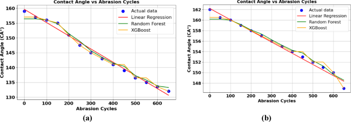
Figure 1a represents the distribution of experimental values (in blue) and values predicted using linear regression, Random Forest and XG Boost ML models for Ni-MA coatings (red, green and yellow, respectively). Key performance metrics were then extracted and reported in Table 1, which included the mean squared error (MSE) and R-squared (R²) values. The MSE measured the average squared differences between the predicted and actual CA values, serving as an indicator of prediction accuracy, while, the R² value represented the proportion of variance in CA that the model explained. Performance metrics for both models are summarized in Table 2, highlighting their effectiveness in forecasting the CA.
The Linear Regression model exhibited excellent performance, with an R² of 0.9979 and a low MSE of 0.229 on the testing data, indicating a near-perfect fit and a strong predictive power. The training data results were also impressive, with an R² of 0.9846 and an MSE of 1.118, suggesting that while the model performed well, it slightly underperformed on the training data compared to the testing set. This highlights the model ability to generalize effectively to unseen data while maintaining a good fit to the training data. In contrast, the Random Forest model showed a slightly higher MSE of 3.00976 on the testing data and an R² of 0.9719. While this is still a strong performance, it is less accurate than Linear Regression in terms of generalization to the testing data. However, the model performed well on the training data, with an MSE of 0.490 and an R² of 0.9933, suggesting that it was able to fit the training data very well. The difference between the training and testing performance indicates a potential overfitting of the Random Forest model to the training data. The XGBoost model, although powerful, demonstrated the highest testing MSE of 3.4182 and an R² of 0.9690, indicating slightly lower accuracy compared to both Linear Regression and Random Forest. On the training data, XGBoost performed exceptionally well, with an MSE of 0.100 and an R² of 0.999, suggesting that the model closely fits the training data. However, similar to Random Forest, this discrepancy in performance between training and testing data points to potential overfitting. Overall, Linear Regression provided the best balance of accuracy and generalization, with superior performance on both training and testing datasets. While Random Forest and XGBoost also demonstrated strong predictive capabilities, they showed a tendency to overfit the training data, leading to slightly reduced performance on the testing data.
Distribution of predicted and measured contact angle values from linear regression, random forest and Xgboost for (a) Ni-MA and (b) Ni-G-MA.
Similar considerations can be drawn on data related to Ni-G-MA coatings, reported in Fig. 1b, whose figures or merit are summarized in Table 3. Indeed, also in this case Linear Regression achieved the highest testing R² with a value of 0.9932 and a low MSE of 0.1557, indicating strong generalization and accuracy. Random Forest had a slightly lower testing R² of 0.9421 with a higher MSE of 1.3258, suggesting it made larger prediction errors but still performed well. XGBoost showed the lowest testing R² of 0.9380 and the highest MSE of 1.4181, indicating higher error rates and potential overfitting, despite achieving perfect accuracy on the training data. Overall, Linear Regression outperformed the other models in terms of both accuracy and generalization.
To evaluate the predictive performance and robustness of the selected machine learning models, 5-fold cross-validation was performed using R² (coefficient of determination) and mean squared error (MSE) as evaluation metrics. Among the tested models, linear regression demonstrated the highest accuracy, achieving an average R² of 0.9616 with a low standard deviation of 0.0504, indicating consistent performance across folds. It also yielded the lowest average MSE of 1.3047, confirming its suitability for modeling degradation trends that follow a relatively linear behavior. The Random Forest model also performed well, with an average R² of 0.9557 and MSE of 2.1399, though slightly less accurate and stable than linear regression, possibly due to sensitivity to data noise or moderate overfitting. In contrast, XGBoost showed comparatively lower performance, with an average R² of 0.8697 and a higher MSE of 5.4084. Additionally, its larger standard deviations in both R² (0.0849) and MSE (1.9493) suggest higher variability and reduced generalization capability. These results indicate that while ensemble models like Random Forest and XGBoost offer flexibility, simpler models such as linear regression may be more effective when the underlying data trends are predominantly linear, offering more reliable and interpretable predictions.
Data augmentation for XGBoost and RF
Data augmentation was applied to the XGBoost and Random Forest models to mitigate overfitting and improve model performance. Among the different augmentation techniques available, Gaussian noise augmentation was selected for its simplicity, effectiveness, and ability to improve model performance. By adding small, controlled random perturbations, it helps prevent overfitting and increases the model exposure to varied data without altering the underlying structure. Unlike methods like SMOTE or jittering, Gaussian noise is easy to apply to both features and targets in regression tasks. It offers precise control over the noise level, allowing for fine-tuning based on model needs. This approach is computationally efficient, scalable, and ideal for situations where generating large datasets is impractical. Gaussian Noise Augmentation involves augmenting a given data point or feature vector, represented as (:x:), by introducing Gaussian noise. Mathematically, this augmentation process can be expressed as39,
$$x_{{augmt}} = x + in$$
(5)
Where:
(:{x}_{augmt:}): represent the augmented data point.
x : is the original data point.
(in): is a random sample drawn from a Gaussian distribution with a mean of 0 and a specified standard deviation.(sigma ~)
The Gaussian distribution is defined as,
$$pleft( in right) = frac{1}{{sqrtleft( {2pi sigma ^{2} } right)}}e^{{ – frac{{ in ^{2} }}{{2sigma ^{2} }}}}$$
(6)
The parameter (:sigma::)specifies the level of noise that is added using Gaussian Noise Augmentation. Smaller values of (:sigma::)indicate reduced noise, whereas larger values of (:sigma::)result in more pronounced noise. In this study, a mean of 0 and a variance of 0.2 are used as Gaussian distribution parameters.
As reported in Tables 4 and 5, data augmentation using Gaussian noise resulted in improved R² scores and reduced MSE for all three models, especially in the testing data. This suggests that augmenting the dataset with Gaussian noise helped the models generalize better by exposing them to a wider variety of data points, thus reducing overfitting. The slight improvements in the testing performance for Linear Regression and Random Forest highlight the benefits of adding augmented data, particularly when real-world data is limited or costly to acquire. XGBoost showed a more dramatic improvement in training performance, indicating that it might have been overfitting to the original data, and Gaussian noise helped alleviate that issue, leading to better generalization on unseen data.
The Table 6 show that Linear Regression outperforms both Random Forest and XGBoost in terms of generalization, with the lowest testing MSE (0.1582) and a high R² (0.9933). This indicates that it provides accurate predictions without overfitting. In contrast, Random Forest and XGBoost exhibit higher testing MSE values (1.3125 and 1.4085, respectively) and lower testing R², suggesting they struggle more with generalization. Notably, XGBoost has an almost perfect training R² (0.9999) and an extremely low training MSE (0.000779), indicating overfitting, where the model memorizes training data but does not perform as well on new data.
Table 7 Figure S3 further confirms these trends, as Linear Regression closely follows the experimental CA values, while Random Forest and XGBoost show minor deviations, particularly at higher abrasion lengths. For example, at 650 mm, the experimental CA is 147, but Random Forest predicts 150, and XGBoost predicts 148, highlighting their slightly reduced accuracy. These results suggest that while all models perform reasonably well, Linear Regression remains the most reliable choice for this dataset, balancing both accuracy and generalization effectively.
To assess the generalization performance of the models, 5-fold cross-validation was conducted using mean squared error (MSE) and R² as evaluation metrics. Linear Regression outperformed the other models, achieving the lowest cross-validated MSE of 0.5355 and the highest R² of 0.9704, indicating excellent predictive accuracy and minimal error on unseen data. Random Forest followed with a higher MSE of 1.3847 and an R² of 0.9235, reflecting good but slightly less consistent performance. XGBoost showed the highest MSE at 1.8816 and the lowest R² of 0.8961 among the three, suggesting that while it can capture complex patterns. Overall, the results highlight that linear regression is the most suitable model for this dataset, likely due to the largely linear nature of contact angle degradation trends under the tested conditions.
Other ML models
Other models were applied to NI-MA and NI-G-MA CA values on different abrasion cycles to capture the corelation between input and output. Result of MSE and R2 are listed in Table 8, Fig. 2.
Table 8 summarizes the performance of various regression models in predicting the contact angle (CA) variation with abrasion length for Ni-MA coatings. Among them, the third-order polynomial regression demonstrated the highest accuracy, with the lowest mean squared error (MSE: 0.2988) and the highest coefficient of determination (R²: 0.9973), indicating a near-perfect fit. The second-order polynomial model also performed well (MSE: 1.8579, R²: 0.9831), capturing the overall trend effectively. However, the fourth-order polynomial exhibited a slightly higher error (MSE: 2.1525, R²: 0.9805), possibly due to overfitting. In contrast, the support vector regression (SVR) model showed poor predictive capability (MSE: 61.6268, R²: 0.4409), likely due to its sensitivity to the dataset’s complexity. The k-nearest neighbours (KNN) model performed better (MSE: 3.7870, R²: 0.9656) but still lagged behind polynomial regression. KNN’s performance is influenced by the choice of neighbours (k) and its reliance on local interpolation. Since CA variation with abrasion length follows a continuous nonlinear trend, KNN’s distance-based approach may fail to generalize well across the entire dataset, leading to inconsistencies. Moreover, KNN is sensitive to noise, and the presence of abrupt changes in CA values can distort its predictions while SVR relies on finding a hyperplane that maximizes the margin within a specified tolerance (epsilon-tube) around the data points, which makes it highly sensitive to the choice of hyperparameters such as kernel type, regularization parameter (C), and epsilon value. If these parameters are not carefully tuned, the model may struggle to capture highly nonlinear patterns, as seen in CA variation with abrasion length. Additionally, SVR assumes that small deviations within the epsilon range are not significant, which might limit its accuracy in datasets where small variations are critical.
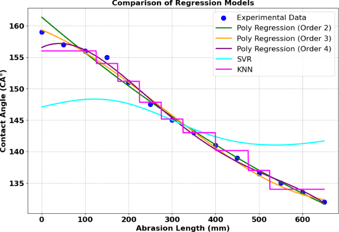
Distribution of predicted and measured contact angle values from polynomial regression order 2,3,4, SVR and KNN models for Ni-MA.
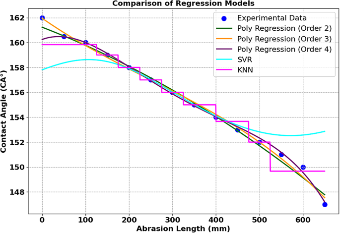
Distribution of predicted and measured contact angle values from polynomial regression order 2,3,4, SVR and KNN models for Ni-G-MA.
In the Table 2 the second-order polynomial regression model achieved a good fit with an MSE of 0.2993 and an R² of 0.9869, capturing most of the data variation. The third-order polynomial regression performed the best, with an exceptionally low MSE of 0.0428 and a high R² of 0.9981, showing high predictive accuracy. In contrast, the fourth-order polynomial regression showed a higher MSE of 1.0509 and a lower R² of 0.9541, suggesting overfitting as the model increased complexity. The Support Vector Regression (SVR) model exhibited the highest MSE of 6.6876 and an R² of 0.7078, indicating poor performance likely caused by its sensitivity to noise and lack of proper tuning. The K-Nearest Neighbours (KNN) model showed moderate results, with an MSE of 2.3056 and an R² of 0.8993, which was better than SVR but still behind the polynomial models.
In Fig. 3 the CA distributions obtained using polynomial regression order 2,3,4, as well as the models and KNN, are presented for Ni-G-MA. Overall, the third-order polynomial regression model outperformed the others. Indeed, the polynomial regression model, especially of order 3, effectively captured the nonlinear relationships within the data, which is crucial for the accurate prediction of contact angles. Compared to other models, Polynomial Regression (Order 3) demonstrated a better balance between bias and variance, as it did not overfit to the training data, unlike models such as XGBoost, which showed overfitting with a perfect training R² but a poor R² on testing data. While Linear Regression also performed well, it did not fully capture the complexities of the dataset, and models like SVR and KNN yielded lower performance in terms of R² and MSE. Therefore, Polynomial Regression (Order 3) stands out due to its ability to model the data underlying patterns more effectively and with greater accuracy. Polynomial regression, particularly the second- and third-order models, performed best because they effectively captured the dataset’s nonlinear pattern without excessive complexity. The fourth-order polynomial suffered from overfitting. SVR performed the worst, likely due to improper tuning and sensitivity to noise, while KNN showed decent but not outstanding performance due to its reliance on local neighbourhood relationships rather than an explicit global function.
The performance of various regression models was evaluated using cross-validation to predict the target output. Among the polynomial models, the third-degree polynomial (Poly3) exhibited the best performance with the lowest mean squared error (MSE) of 0.6649 and the highest coefficient of determination (R²) of 0.9918, indicating a strong fit to the data. In comparison, Poly2 and Poly4 showed slightly higher MSE values of 1.2249 and 1.2924, with corresponding R² values of 0.9849 and 0.9840, respectively. The k-nearest neighbors (KNN) model also demonstrated good predictive accuracy with an MSE of 3.5675 and an R² of 0.9559. However, the support vector regression (SVR) model yielded significantly poorer results, with a high MSE of 46.4255 and a low R² of 0.4262, indicating limited suitability for this dataset. Overall, the Poly3 model emerged as the most reliable among the tested algorithms.
Tape peeling and chemical stability datasets
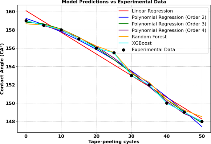
The dataset presented in Table S3, Table S4 was analysed to investigate the relationship between the contact angle (CA) and tape peeling cycles. To achieve this, various modelling techniques were applied, including linear regression, polynomial regression, XGBoost, and Random Forest, as illustrated in Fig. 6. For capturing potential nonlinear relationships, polynomial regression models of degrees 2 through 4 were utilized, offering enhanced flexibility to accurately represent complex patterns within the data. Advanced ML models, such as XGBoost and Random Forest, were also employed as their ability to handle intricate, nonlinear associations effectively. These approaches provided a robust framework to complement traditional regression methods, enabling a more comprehensive understanding of the underlying trends in the dataset.
Table 9 presents the Mean Squared Error (MSE) and R² values for different regression models applied to Ni-MA data. The results indicate that the XGBoost model outperforms all others, achieving the lowest MSE (0.0001) and the highest R² (0.9999), demonstrating its superior predictive accuracy. Random Forest and higher-order Polynomial Regression models also exhibit strong performance, with R² values exceeding 0.99, while Linear Regression has the highest MSE (0.4090), suggesting a weaker fit. The trend highlights the advantage of non-linear models in capturing complex relationships within the data, with XGBoost providing the most precise predictions (Fig. 4).
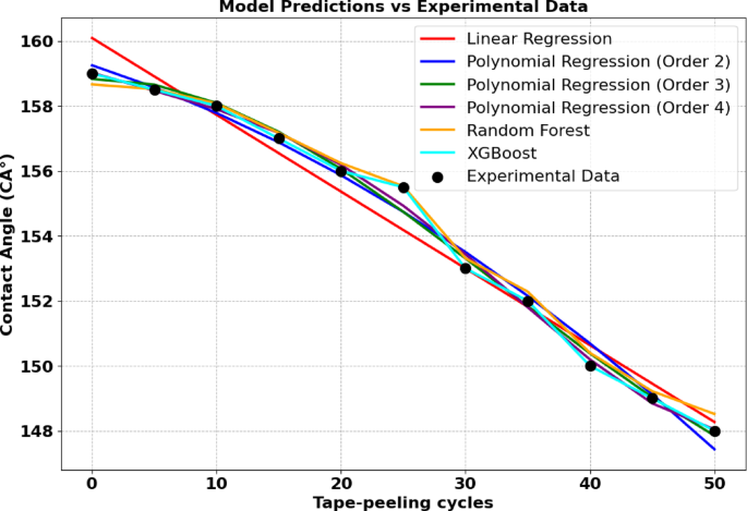
Distribution of predicted and measured contact angle values from linear regression XGBoost, Random Forest, poly order 2,3,4 for Ni-MA.
In Table 10; Fig. 5, the results illustrate the effectiveness of various models in predicting the CA based on tape-peeling cycles. Linear regression performed well, with an MSE of 0.1161 and an R² of 0.9931, capturing the overall linear trend in the data. However, nonlinear models offered better flexibility in identifying subtle patterns. Polynomial regression models demonstrated significant improvements, with the second-order model achieving an MSE of 0.1159 and an R² of 0.9932, while the third- and fourth-order models further enhanced predictions, both achieving an MSE of 0.0620 and an R² of 0.9963. Advanced machine learning techniques were also applied, with Random Forest achieving an MSE of 0.1561 and an R² of 0.9908, effectively modelling the dataset’s nonlinear features. The XGBoost model outshone all others, achieving an outstandingly low MSE of 0.00098 and an R² of 0.999, underscoring its ability to model complex relationships with exceptional accuracy and reliability. While polynomial regression and Random Forest provided strong performance, XGBoost proved to be the most accurate and versatile model.
Distribution of predicted and measured contact angle values from linear regression XGBoost, Random Forest, poly order 2,3,4 for Ni-G-MA.
The comparative evaluation of regression models using 5-fold cross-validation revealed that polynomial regression models outperformed other approaches in terms of prediction accuracy. Specifically, the fourth-order polynomial regression model achieved the best performance, with the lowest mean squared error (MSE) of 0.1674 and the highest coefficient of determination (R²) of 0.9884. This was closely followed by the third-order polynomial model (MSE: 0.1951, R²: 0.9864), indicating that increasing the polynomial order up to a certain extent improves model fit. The second-order polynomial and linear regression models also showed strong performance, with R² values of 0.9704 and 0.9640, respectively. In contrast, ensemble models such as Random Forest and XGBoost demonstrated relatively lower predictive accuracy, with MSE values of 0.7424 and 1.4772, and corresponding R² values of 0.9484 and 0.8972. These findings confirm the effectiveness of polynomial regression, particularly of orders three and four, in capturing the underlying patterns in the dataset.
In the dataset presented in Table S5, S6 we begin the analysis by plotting the CA against the number of sand impact cycles. To show the relationship between these variables, we employ a combination of polynomial regression, linear regression, XGBoost, and Random Forest models.
Table 11 presents the Mean Squared Error (MSE) and R² values for Ni-MA modeling using Linear Regression, Random Forest, and XGBoost. The Linear Regression model demonstrates the best performance with the lowest MSE (0.1336) and highest R² (0.9863), indicating strong predictive accuracy and minimal error. The Random Forest model shows slightly higher error (MSE = 0.3162) and a lower R² (0.9675), suggesting a moderate decrease in performance. In contrast, the XGBoost model exhibits significantly higher MSE (1.4160) and lower R² (0.8544), indicating a poorer fit, due to overfitting, hyperparameter tuning issues.
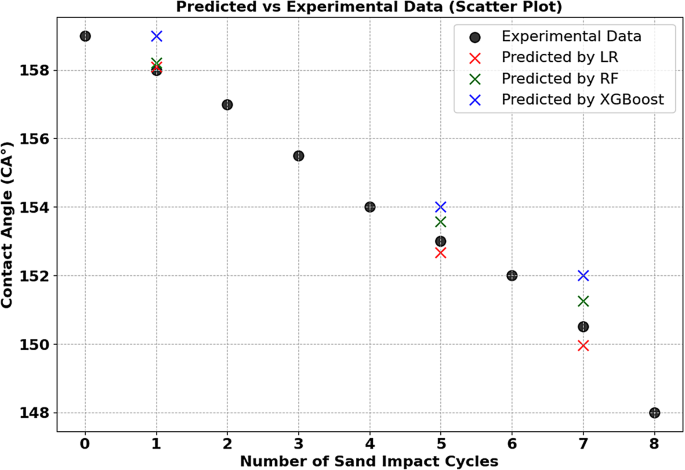
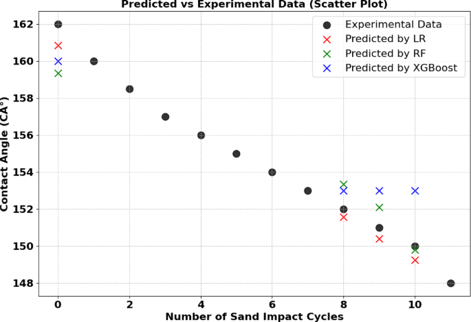
Figure 6 presents a scatter plot comparing the predicted and experimental contact angles (CA°) as a function of the number of sand impact cycles. The black dots represent experimental data, while predictions from Linear Regression (LR), Random Forest (RF), and XGBoost models are indicated by red crosses, green crosses, and blue crosses, respectively.
The plot shows that Linear Regression and Random Forest predictions closely align with the experimental values, particularly at lower sand impact cycles, reinforcing their superior performance (as indicated by the lower MSE and higher R² values in Table 11). In contrast, the XGBoost model exhibits greater deviations, especially at higher impact cycles,
Distribution of predicted and measured contact angle values from linear regression XGBoost, Random Forest, for Ni-MA.
In Table 12; Fig. 7, the Linear Regression model is the best, with the lowest MSE (0.1250) and highest R² (0.9945), showing it fits the data most accurately. The other models, Random Forest and XGBoost, have higher MSE and lower R² values, suggesting less accurate predictions.
Distribution of predicted and measured contact angle values from linear regression XGBoost, Random Forest, for Ni-G-MA.
The 5-fold cross-validation analysis further highlights the superiority of linear regression for this dataset. Linear regression achieved the lowest mean squared error (MSE) of 0.2820 and the highest coefficient of determination (R²) of 0.9826, indicating an excellent fit and strong predictive capability. In contrast, ensemble models such as Random Forest and XGBoost showed relatively lower performance, with MSE values of 1.6400 and 2.2089, and R² values of 0.8987 and 0.8635, respectively. Although ensemble techniques are generally robust for complex, non-linear data, in this case, the simplicity of linear regression appears to better capture the underlying relationships, likely due to the dataset’s linear or near-linear characteristics.
In Table S7, S8 we analyse the relationship between the CA and number of days in NaCl (0.5 M) solution by plotting the data and applying again various machine learning models.
Distribution of predicted and measured contact angle values from linear regression, XGBoost, Random Forest, for Ni-MA.
Cross-validation (5-fold) was conducted to evaluate the performance and generalization capability of different regression models. Linear regression exhibited the best performance among the evaluated models, with a mean squared error (MSE) of 0.1887 ± 0.1297. Random Forest and XGBoost showed significantly higher errors, with MSE values of 2.1400 ± 1.3269 and 3.8006 ± 0.9731, respectively.
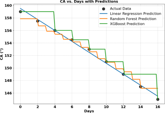
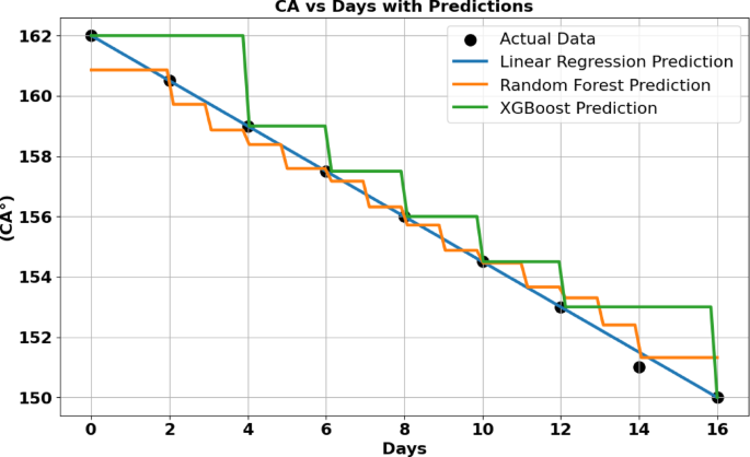
Figure. 8 illustrates the variation of contact angle (CA°) over time of immersion in NaCl (days) using actual data (black dots) and predictions from three models: Linear Regression (blue line), Random Forest (orange line), and XGBoost (green line). The Linear Regression model follows a smooth, linear trend, closely approximating the overall experimental pattern. The Random Forest and XGBoost models, in contrast, exhibit step-like predictions, characteristic of tree-based models. While Random Forest predictions align relatively well with actual data, XGBoost shows larger deviations, particularly at certain intervals, reinforcing its higher MSE (3.1235) and lower R² (0.8867) Table 13. This suggests that XGBoost struggles with the dataset’s characteristics, potentially due to overfitting or sensitivity to variations in the data.
In Table 14; Fig. 9, considering the same phenomenon on coating Ni-G-MA, the Linear Regression model is the best, with the lowest MSE (0.1250) and highest R² (0.9945), showing it fits the data most accurately. The other models, Random Forest and XGBoost, have higher MSE and lower R² values, suggesting less accurate predictions.
Distribution of predicted and measured contact angle values from linear regression XGBoost, Random Forest, for Ni-G-MA.
ML models were also applied to data in Table S9, S10 to find out correlation between CA and number of days of exposure in open environment.
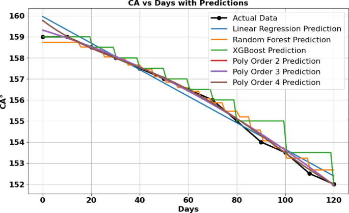
Table 15; Fig. 10 compare the performance of various models in predicting contact angle values after outdoor exposure in coating Ni-MA. The Polynomial Regression models of order 2 and 3 achieve the best results with the lowest MSE (0.1125) and highest R² (0.9854), indicating excellent predictive accuracy. Random Forest also performs well (MSE = 0.3085, R² = 0.9601), outperforming Linear Regression (MSE = 0.4228, R² = 0.9452) and XGBoost (MSE = 0.6668, R² = 0.9137). The fourth-order polynomial model (MSE = 0.2446, R² = 0.9683) shows slight overfitting, suggesting that a second- or third-order polynomial is optima for this dataset.
Distribution of predicted and measured contact angle values from linear regression XGBoost, Random Forest, for Ni-MA.
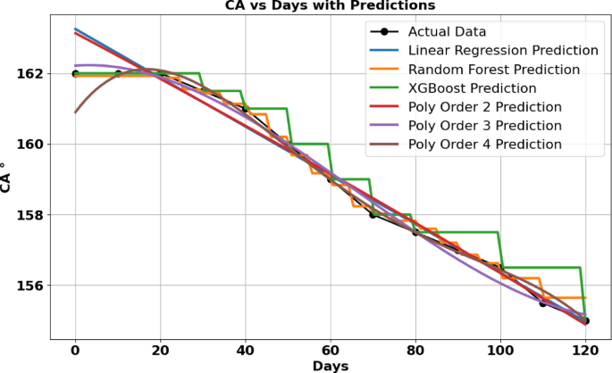
In Table 16 Fig. 11, when applying the models to outdoor exposure of coating Ni-G-MA, the Polynomial Regression of Order 3 performs the best, with the lowest MSE (0.0393) and the highest R² (0.9949). This indicates a very close fit to the data, capturing the underlying relationship with high accuracy. Polynomial Regression of higher orders (4) and other models, such as Random Forest and XGBoost, show slightly worse performance, likely due to overfitting (in the case of higher polynomial orders) or a less optimal fit compared to the cubic model. The Linear Regression also performs reasonably well, but its MSE and R² indicate it doesn’t capture the more complex relationship as effectively as the cubic polynomial.
Distribution of predicted and measured contact angle values from linear regression XGBoost, Random Forest, for Ni-G-MA.
A detailed 5-fold cross-validation was performed to assess the predictive accuracy and stability of multiple regression models. Among all models, polynomial regression of order 2 demonstrated the best performance, achieving the lowest mean squared error (MSE) of 0.0566 ± 0.0506 and the highest mean R² value of 0.9866 ± 0.0081, indicating excellent fit and low variance across folds. Polynomial regressions of orders 3 and 4 followed closely, with MSEs of 0.0601 and 0.0771 and R² values of 0.9797 and 0.9796, respectively, suggesting that higher-order terms do not significantly enhance model performance beyond the second order. Among the non-polynomial models, Random Forest outperformed both Linear Regression and XGBoost, achieving an MSE of 0.2291 ± 0.1916 and R² of 0.9333 ± 0.0385. Linear Regression yielded a mean MSE of 0.1855 ± 0.1269 and R² of 0.9025 ± 0.0902, while XGBoost showed the lowest performance with an MSE of 0.3667 ± 0.1869 and R² of 0.8094 ± 0.1477. Overall, these results clearly indicate that second-order polynomial regression offers the best balance of accuracy and generalizability for this dataset.
Eventually, concerning data related to coatings immersion in different pH and reported in Table S11, S12, all models struggle to predict contact angle (CA) at different pH levels, with high MSE values and mostly negative R² scores, likely due to the small dataset failing to capture underlying patterns. Among them, the fourth-order polynomial model (Poly Order 4) performs relatively better, achieving the lowest MSE (0.4118) and the only positive R² (0.5882). However, despite its improved fit compared to other models, its predictive accuracy remains suboptimal, suggesting that the dataset lacks sufficient variation for reliable trend identification Figure S4.
Stability prediction on superhydrophobic coatings
In this study, we employed a variety of machine learning (ML) and regression models, including XGBoost, K-Nearest Neighbours (KNN), Random Forest (RF), Support Vector Regression (SVR), and multiple polynomial regression models, to predict the stability of the contact angle (CA) under different environmental and mechanical stress conditions. These conditions included immersion in NaCl solution, varying abrasion cycles, tape peeling tests, sand impact, and open-air exposure. Our analysis revealed that the best-performing model varied depending on the specific degradation mechanism. For abrasion cycles and tape peeling tests, linear regression performed best, as the CA degradation followed a relatively linear trend due to gradual surface wear and adhesive forces. XGBoost also demonstrated strong predictive capability in these cases, benefiting from its ability to detect slight nonlinearities while remaining robust against noise. However, for sand impact and open-air exposure, where the CA degradation followed a nonlinear trend, third-order polynomial regression (cubic regression) outperformed other models. The nature of sand impact resulted in an initial sharp decline in CA followed by stabilization, while open-air exposure led to a time-dependent degradation influenced by oxidation and contamination effects. Higher-order polynomial regression effectively captured these nonlinear trends, whereas simpler models like linear regression and SVR failed to generalize well. Among all models, XGBoost consistently delivered strong performance across multiple conditions, as it could handle both linear and nonlinear relationships while effectively reducing overfitting. In contrast, SVR and KNN exhibited weaker predictive capabilities. SVR struggled due to its sensitivity to hyperparameter tuning, leading to suboptimal performance in highly nonlinear cases such as sand impact and open-air exposure. KNN, being a distance-based algorithm, was less effective at capturing long-term trends and tended to overfit localized variations, making it unsuitable for extrapolating CA degradation over extended periods.
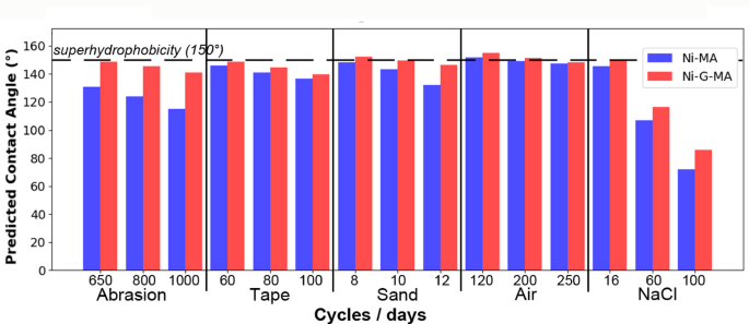
Using the best-performing model in each case, the contact angle (CA) values were predicted under different untested conditions, as shown in Figure. 12. These predicted values closely match the experimental results until available (Figure S5, S6 Table S13), confirming the model reliability in estimating CA under different environmental and mechanical conditions. Moreover, these values allow to draw conclusions on the long-term behavior of these coatings, indicating that Ni-G-MA overperforms Ni-MA. to the presence of graphene not only in initial conditions, but also by preserving, or approaching, superhydrophobicity on a longer run even when subjected to strong mechanical stress. The only clear point of failure of superhydrophobicity for both coatings was for prolonged contact with salty water, which indeed is one of the major concerns in the field of coatings durability.
Predicted contact angle values from linear for Ni-MA and Ni-G-MA.
Based on the predicted contact angle data), NaCl immersion emerged as the most critical degradation factor, especially over prolonged exposure (100 days), where both Ni-MA and Ni-G-MA coatings experienced a substantial drop in contact angle falling below the 150° superhydrophobic threshold. In contrast, air storage, sand impingement, and tape peeling exhibited relatively minor influence, with contact angles consistently remaining above 150°, indicating better stability under those conditions. Notably, abrasion resistance was improved in Ni-G-MA compared to Ni-MA, suggesting that graphene incorporation enhanced mechanical robustness. This analysis highlights chemical durability particularly in corrosive environments as the most significant challenge to maintaining long-term superhydrophobicity, and has been discussed in detail in the revised manuscript.
Linear Regression was chosen as a baseline due to its simplicity and interpretability. Polynomial Regression (orders 2–4) was applied to capture potential non-linear relationships between the input features and the predicted contact angle. Random Forest and XGBoost, both ensemble-based models, were selected for their ability to model complex, non-linear interactions and their robustness to overfitting. These models are widely used in materials science and surface engineering for predictive tasks due to their high accuracy and feature importance analysis capabilities.