Study population and dataset
The CHARLS is a prospective national cohort study that enrolled 17,708 participants in 2011, and three waves of follow-up were conducted in 2013, 2015, and 2018. Participants were randomly selected using a probability-proportional-to-size (PPS) technique and a four-stage random sample method. The workgroup selected 150 counties in 28 provinces. Administrative villages in rural areas and neighborhoods in urban areas were the primary sampling units (PSUs). Three PSUs within each county-level unit were selected using PPS sampling. Detailed information on the methodology and cohort profile has been reported previously [11].
We collected data on participants enrolled in the baseline investigation who attended all three follow-up investigations and aged above 60 years old. Those with a history of cancer were excluded because the progression and treatment of cancer affect multiple organs and systems throughout the body; this aspect could have introduced substantial bias into our study. During the data cleaning process, we identified participants with implausible data regarding body weight and height, specifically heights less than 100 cm or weights less than 20 kg. These values were considered erroneous owing to likely data entry mistakes; therefore, participants with an abnormal body mass index (BMI) (BMI < 10 or BMI > 60) in the baseline investigation were excluded.
Altitude data acquisition
The participants’ place of residence was determined by their community ID. The latitude and longitude were acquired through amap api (https://restapi.amap.comv3/geocode), and the local altitude was acquired based on the latitude and longitude using geodata (version 0.5-8) [12] packages and the raster package (version 3.6–23) [13]. Participants were stratified into a low-altitude or high-altitude group based on a criterion of 1500 m, which was used in previous studies [14].
Variable collection
The primary outcome was hip fractures reported by the participants, which was defined by their answer to the question, “Have you fractured your hip since the last interview?” Participants choosing “yes” were considered to have experienced a hip fracture, and the time point the investigation occurred was recorded as the time the event happened.
Individual income, marital status, medical history, sex, BMI, smoking status, alcohol consumption, and age were selected as covariates for propensity score matching (PSM). Individual income was acquired from harmonized CHARLS data and evenly divided into five groups. Educational status was retrieved from the answer to the question: “What is the highest level of education completed?” and re-coded into preschool, primary, secondary, and higher education. Marital status was retrieved from the answer to the question: “What is your marital status?” and re-coded as unmarried, married, widowed, divorced (or long-term separation). History of stroke, cardiovascular dysfunction, falls, hip fractures, chronic lung diseases, and arthritis were retrieved from the answer to the question: “Have you been diagnosed with any of the following by a doctor?” The presence of specific diseases was determined based on whether the participant selected “Yes” to the following conditions: (1) “Chronic lung diseases, such as chronic bronchitis and emphysema (excluding tumors or cancer),” (2) “Heart attack, coronary heart disease, angina, congestive heart failure, or other heart problems,” (3) “Stroke,” and (4) “Arthritis or rheumatism.” BMI was calculated using the following formula: BMI (kg/m[2]) = body weight (kg)/body height (m)2.
Propensity score matching
Individual income, marital status, medical history, sex, BMI, smoking status, alcohol consumption, and age were selected for PSM. A general linear model was used to calculate the distance, and the nearest method was used for matching with a matching ratio of 1:8 (high altitude: low altitude). After matching, a balance test was performed to evaluate the imbalance between the two groups in the matched data. The MatchIt package [15] was used for matching, and the Cobalt package [16] was used for the balanced test and plotting.
Statistical analysis
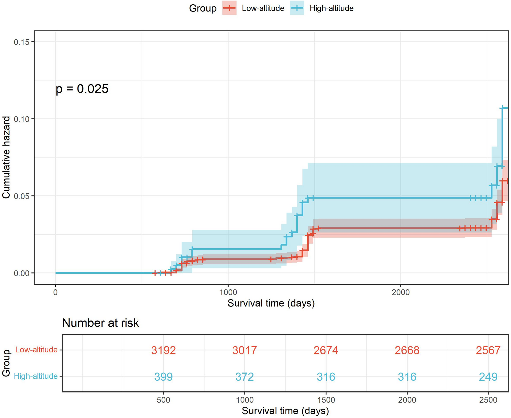
Categorical variables are shown as counts (percentages, %), and continuous variables are shown as mean ± SD. To compare the differences in baseline data between the two groups, chi-square and t-tests were used for categorical and continuous variables, respectively. Kaplan–Meier survival analysis and Cox regression were used to compare the differences between the two groups regarding fall and hip fracture risks.
Subgroup analysis was performed, and the participants were divided into subgroups according to sex, smoking history, and overweight status. The effects of high-altitude exposure on fall and hip fracture risks in different subgroups were evaluated using Cox regression analysis.
To test the robustness of our results, we performed different sensitivity analyses as follows: (1) We randomly sampled 80% and 90% of all participants, respectively, and replicated the previously described analysis workflow. (2) Using optimal matching as the PSM method and a matching ratio of 1:8, we replicated the previously described analysis workflow. (3) Cox regression was performed with and without adjustments for covariates without matching the participants.
All analyses were performed using R (version 4.3.1). The survival analysis was performed using the survival package (version 3.5-5) [17] and visualized using the Survminer package (version 0.4.9) [18]. The comparison of baseline characteristics and the generation of tables was performed using the gtsummary package (version 1.7.2) [19].