Data collection
Statistical data
This study collected agricultural statistical data at the national, provincial, prefectural, and county levels in China, covering the period from 1988 to 2022. The data sources include the statistical yearbooks from the National Bureau of Statistics of China (https://www.stats.gov.cn) and the Big Data Research Platform for China’s Economy and Society (https://data.cnki.net). Moreover, historical crop price records were obtained from the FAO (Food and Agriculture Organization of the United Nations) (https://www.fao.org/faostat)41. To evaluate irrigation and agricultural input levels, crop fertilizer application ratios were derived from the inventories of “Compilation of the National Agricultural Costs and Returns”42. Recommended fertilizer application ratios for different crops were obtained from He et al.43. The proportion of irrigated land was obtained from the third simulation round of the Inter-Sectoral Impact Model Intercomparison Project (ISIMIP3a) dataset44, which provides data on rainfed and irrigated cropland for crops from 1901 to 2021.
Spatial data
Several spatial datasets relevant to crop distribution, including land use, crop natural growth suitability, urban boundaries, and population density, have been used to facilitate the mapping of crop area. The land use data were employed to delineate the extent of cropland and irrigated cropland, including the China Land Cover Dataset (CLCD)45, the China Land Use and Land Cover Remote Sensing Monitoring Dataset (CNLUCC)46, the Global Land Cover Fine-Grained Classification Product (GLC_FCSD)47, the China Arable Land Dataset (CACD)3, and the China Irrigated Cropland Dataset48. The crop natural growth suitability and potential yield distribution were derived from the GAEZ v4 dataset49. The population density data originated from the China Population Spatial Distribution Dataset50. The urban extent data were obtained from the China Urban Boundary Dataset (GAIA)51. Additionally, the transport accessibility data were obtained from Weiss et al.52. All spatial datasets were rasterized and resampled to a 1-km resolution grid. The details of these datasets are provided in Table 1.
Modeling framework
The research framework is illustrated in Fig. 2, which consists of four key steps: pre-processing statistical and spatial data, allocating statistical harvest area data, validating the accuracy of the results, and analyzing spatiotemporal changes of crop patterns. First, national, provincial, and prefectural statistical data were harmonized and downscaled to grids, while county-level data were used to validate the accuracy of the mapping results. Then, crop cultivation was categorized into three different production systems, i.e., irrigated, high-input rainfed, and low-input rainfed based on crop irrigation and fertilizer application ratios. Multiple land use datasets were then integrated to develop a synthetic map of cropland and irrigated cropland. Meanwhile, pre-processing was performed on spatial datasets such as city boundaries, population distribution, and transportation accessibility (Figs. S1–S3). Then, a spatial allocation framework was used to downscale the prefecture-level crop area statistics into 1-km grids. Moreover, the accuracy of the dataset was evaluated in terms of both validation metrics and spatial patterns. Finally, changes in the spatiotemporal heterogeneity of crop distribution were analyzed.
Harmonization of statistical data
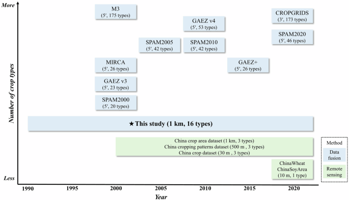
This study collected harvest area statistics for 16 different crop types across four different political administration levels. The detailed list of crop names is provided in Table 2. The time coverage of this built dataset spans from 1990 to 2020. We endeavored to collect crop statistics from publicly accessible sources, generally ensuring data completeness for major production regions (Fig. S4). However, due to the extended temporal coverage and reliance solely on public data, many regions inevitably have incomplete time series. To ensure data availability and methodological consistency, we followed previous studies by representing each time point with a 5-year average, using data from the two years before and after each time point26,29,53,54. For instance, statistical values from 1988 to 1992 were utilized to map the crop patterns in 1990, while those from 2018 to 2022 were employed to map the crop patterns in 2020. Besides, the linear interpolation was used to fill the missing values. Due to the lack of prefecture-level statistical data for Xinjiang, Qinghai, and Xizang, spatial allocations for these provinces were based on provincial-level statistical data.
In order to ensure the consistency of statistical data across different administrative levels, this study used national-level statistical data as a benchmark and successively corrected for each province and prefecture. First, the crop harvest area for each province (({{HA}}_{j,t,p}^{{stat}})) was adjusted according to Eq. (1), based on the national total harvest area (({{HA}}_{j,t,{national}}^{{stat}})), resulting in the revised provincial harvest area denoted as ({{HA}}_{j,t,p}^{{revise}}):
$${{HA}}_{j,t,p}^{{revise}}={{HA}}_{j,t,p}^{{stat}}times frac{{{HA}}_{j,t,{national}}^{{stat}}}{sum _{p}{{HA}}_{j,t,p}^{{stat}}},$$
(1)
where the j denotes the crop type, t represents the time node, and p indicates the provincial-level administrations. The sum of the revised area at the provincial level is highly in agreement with the national statistics, as shown in Fig. S5.
Based on the revised provincial-level data, a similar approach is applied to adjust the harvest area for the prefecture-level city (({{HA}}_{j,c}^{{stat}})) as Eq. (2):
$${{HA}}_{j,t,c}^{{revise}}={{HA}}_{j,t,c}^{{stat}}times frac{{{HA}}_{j,t,p}^{{revise}}}{sum _{c}{{HA}}_{j,t,c}^{{stat}}},$$
(2)
where the (c) represents the prefecture-level city with province (p). The sum of the harmonized data at the prefecture level is equal to the revised provincial values, as shown in Fig. S6. Therefore, the total harmonized harvest area of all provinces and prefectures equals the national statistics.
Classification of crop production systems
Based on the ratios of irrigation and fertilizer application, each crop cultivation was categorized into three production systems: irrigated, high-input rainfed, and low-input rainfed. The proportion of irrigated crop for each 5-year node was extracted from the ISIMIP3a dataset44. The proportions of high-input and low-input systems are determined based on actual crop fertilizer application statistics compared with the recommended amounts. The shares of irrigated system for crops (({H{A}_{{Ratio}}}_{j,t,p}^{{irrigat}{ion}})) are determined by averaging the gridded values at the prefecture level. Owing to the lack of crop fertilizer application data at the prefecture level, this study assumed that all prefectures within the same province share the same average fertilizer application ratios. The details of the crop production system classification are as follows.
First, the crop fertilizer application ratios of each province (({{Fert}}_{j,t,p}^{{unit}})) were obtained from the “Compilation of the National Agricultural Costs and Returns” as presented in Table S2. Then, the sum of fertilizer application for each crop (({{Fert}}_{j,t,p}^{{Sum}})) was calculated using Eq. (3). The average crop fertilizer applications for all provinces are shown in Table S3.
$${{Fert}}_{j,t,p}^{{Sum}}={{HA}}_{j,t,p}^{{revise}}times {{Fert}}_{j,t,p}^{{unit}}$$
(3)
Then, the high-input production area of the crop (({{HA}}_{j,t,p}^{{high}})) is obtained from dividing the total fertilizer application by the recommended fertilizer application ratios for the crop (({{Fert}}_{j,p}^{{recommend}})), as shown in Eq. (4):
$${{HA}}_{j,t,p}^{{high}}=frac{{{Fert}}_{j,t,p}^{{Sum}}}{{{Fert}}_{j,p}^{{recommend}}}.$$
(4)
The ratios of high-input system in the total area (({H{A}_{{Ratio}}}_{j,t,p}^{{high}})) are calculated following Eq. (5):
$${{HA}{rm{_}}{Ratio}}_{j,t,p}^{{high}}=frac{{{HA}}_{j,t,p}^{{high}}}{{{HA}}_{j,t,p}^{{revise}}}.$$
(5)
Finally, the ratios of the low-input system (({H{A}_{{Ratio}}}_{j,t,p}^{{low}})) are calculated by subtracting the proportion of the irrigated and high-input area following Eq. (6). Tables S4–S6 show the detailed proportions for each production system.
$${{HA}{rm{_}}{Ratio}}_{j,t,p}^{{low}}=1-{{HA}{rm{_}}{Ratio}}_{j,t,p}^{{irrigat}{ion}}-{{HA}{rm{_}}{Ratio}}_{j,t,p}^{{high}}$$
(6)
Synthesis of cropland
The cropland distribution from different sources was synthesized using the multi-source data integration approach proposed by Lu et al.55. The cropland extents were obtained from CACD, CLCD, GLC_FCSD, and CNLUCC datasets. The spatial resolutions of these datasets were resampled to 1 km, with temporal periods aligned to the time nodes of the statistics.
First, the average and maximum cropland areas for each grid were derived by spatially overlaying multiple datasets. Then, a ranking scoring table was developed to assess the credibility of the cropland distribution. As shown in Table S7, the agreement level reflects the degree of consensus among the datasets in classifying a grid cell as cropland. The rank value indicates the order of reliability across different data combinations. For example, an agreement level of 4 indicates that all datasets classify the grid cell as cropland; conversely, a value of 1 indicates that only one dataset identifies the cell as cropland. The ranking of the datasets was determined through existing data quality comparison studies and expert judgment. Given that the CACD was specifically developed for cropland mapping, it is considered to have the highest level of credibility56. Additionally, comparative studies on data accuracy indicate that the CLCD demonstrates higher overall accuracy when compared to both the GLC_FCSD and the CNLUCC datasets57,58. Finally, the synthesized average cropland area maps are illustrated in Fig. S7.
The approach for irrigated cropland synthesis is similar to cropland. The irrigated cropland maps were obtained from the China Irrigated Cropland Dataset, GLC_FCSD, and CNLUCC datasets. A scoring table for these irrigated cropland datasets is provided in Table S8. The synthesized maps of average irrigated cropland area for the period from 1990 to 2020 are shown in Fig. S8.
Spatial allocation of crop statistics
Prefecture-level statistics were allocated to 1-km grids using the maximum-score optimization approach developed by van Dijk et al.40. This method builds upon the minimum cross-entropy framework originally proposed by You and Wood (2005, 2006)31,32. The cross-entropy framework calculates the prior probability of crop distribution based on biophysical and socioeconomic factors, and then determines the actual probability under statistical constraints by minimizing cross-information entropy33. To enable multi-temporal, high-resolution mapping, the maximum plant suitability score was used in place of the minimum cross-entropy metric, resulting in improved spatial resolution and faster convergence. The main steps of the model are described below.
First, the crop harvest area of the prefecture (({{HA}}_{j,t,c}^{{revise}})) is converted into the physical area (({{PA}}_{j,t,c})) based on crop planting intensity (({{CropIntensity}}_{j,t,c})) as expressed in Eq. (7). The assumption is that there is no difference in cropping intensity between prefectures within the same province. The average crop planting intensities for different crops are shown in Table S9.
$${{PA}}_{j,t,c}=frac{{{HA}}_{j,t,c}^{{revise}}}{{{CropIntensity}}_{j}}$$
(7)
Then, the crop plant suitability scores for different crop production systems (l) within the grid (i) are calculated. The irrigated and rainfed high-input systems are mainly located in large farms, and their score is influenced by both biophysical characteristics and socio-economic factors, including transport accessibility and crop prices. Therefore, their crop plant suitability score is presented as Eq. (8):
$${{score}}_{i,j,l}=sqrt{{{access}}_{i}times {{rev}}_{i,j,l}},lin left{{irrigation},{rained; high; input}right},$$
(8)
where the ({{access}}_{i}) represents the accessibility from the grid to cities, and where ({{rev}}_{{ijl}}) represents the economic benefit of the crop, which is calculated via Eq. (9):
$${{rev}}_{i,j,l}={{pot}{rm{_}}{yield}}_{i,j,l}times {{price}}_{j},$$
(9)
where the ({{pot_yield}}_{i,j,l}) is the potential yield of crop (j) in grid (i) under (l) system, which is obtained from the GAEZ v4 dataset. The changes in crop prices (({{price}}_{j})) are shown in Table S10.
For rained low-input system, its plant suitability score is constrained mainly by the natural environment, which is calculated following Eq. (10):
$${{score}}_{i,j,l}={s{uit}{rm{_}}{index}}_{i,j,l},lin left{{rained; low; input}right}.$$
(10)
The ({s{uit}{_index}}_{{ijl}}) denotes the plant suitability of crop (j) in grid (i) under (l) system, which is derived from the GAEZ v4 dataset as well.
Finally, based on the plant suitability scores of crops, the objective function designed to maximize the plant suitability score is formulated as Eq. (11):
$$max {sum }_{i}{sum }_{j}{sum }_{l}{s}_{i,j,l}times {{score}}_{i,j,l}.$$
(11)
The ({s}_{i,j,l}) represents the ratio of the area allocated to crop (j) under system (l) to the total area of the grid, which is the target solution value of the model. Meanwhile, the subsequent constraints should be abided by during the model-solving process as indicated in Eqs. (12–16).
-
1.
The area allocated to crops within the grid must not exceed the total area of the grid.
$$0le {s}_{i,j,l}le 1,forall ,iforall ,jforall ,l$$
(12)
-
2.
The cumulative ratios of different production systems within the grid must sum to 1.
$$sum _{l}{s}_{i,j,l}=1,forall ,iforall ,j$$
(13)
-
3.
The crop area is equal to the statistical data.
$$sum _{l}{{PA}}_{j,c}times {s}_{i,j,l}={{PA}}_{j,c},forall ,i$$
(14)
-
4.
The crop area does not exceed the total cropland area within the prefecture (({{cropland}{rm{_}}{area}}_{c})).
$$sum _{l}{{PA}}_{j,l,c}times {s}_{i,j,l}le {{cropland}{rm{_}}{area}}_{c},forall ,iin c$$
(15)
-
5.
The irrigated crop area does not exceed the total irrigated cropland area within the prefecture (({{irrigation_area}}_{c})).
$$sum _{l={irrigation}}{{PA}}_{j,l,c}times {s}_{i,j,l}le {{irrigation}{rm{_}}{area}}_{c},forall ,i$$
(16)
To address data inconsistencies between different types of constraints, the slack variables are incorporated into the objective function. Higher weights (106) are assigned to constraints relating to cropland availability and irrigated area to limit their slack, while lower weights (105) are assigned to constraints relating to subnational statistics. This configuration ensures solution feasibility and quantitatively clarifies trade-offs in constraint prioritization40,59. Furthermore, all weights, parameters, and implementation details have been made publicly available to enable rigorous validation and to ensure the robustness and reproducibility of the results.
The optimization model was implemented in the GAMS (General Algebraic Modeling System) using a linear programming framework, with the CPLEX (C-Simplex algorithm) solver employed to efficiently address large-scale spatial allocation problems. Data exchange between model components was managed by GDX (GAMS Data eXchange) format files. All data preprocessing and visualization procedures were performed in R60. To improve allocation accuracy for China-specific crop patterns, we enhanced the original mapspamc package38, thereby maintaining methodological consistency with global applications.
Validation metrics
The county-level statistics are used to evaluate the accuracy of the allocation results at the prefecture level. The scatter plot illustrates the relationship between the statistically derived harvest area (({{HA}}^{{stat}})) and the allocated harvest area (({{HA}}^{{alloc}})). Meanwhile, the Pearson correlation coefficient ((C{or})), the coefficient of determination (left({R}^{2}right)), and the root mean square error (({RMSE})) is used to quantitatively evaluate the accuracy of the results. The calculation methods for the different accuracy verification metrics are presented in Eqs. (17–19):
$${Cor}({{HA}}^{{alloc}},{{HA}}^{{stat}})=frac{mathop{sum }limits_{k=1}^{n}({{HA}}_{k}^{{stat}}-bar{{{HA}}^{{stat}}})({{HA}}_{k}^{{alloc}}-bar{{{HA}}^{{alloc}}})}{sqrt{mathop{sum }limits_{k=1}^{n}{({{HA}}_{k}^{{alloc}}-bar{{{HA}}^{{alloc}}})}^{2}}sqrt{mathop{sum }limits_{k=1}^{n}{({{HA}}_{k}^{{stat}}-bar{{{HA}}^{{stat}}})}^{2}}},$$
(17)
$${R}^{2}=1-frac{mathop{sum }limits_{k=1}^{n}{left({{HA}}_{k}^{{alloc}}-{{HA}}_{k}^{{stat}}right)}^{2}}{mathop{sum }limits_{k=1}^{n}{left({{HA}}_{k}^{{alloc}}-bar{{{HA}}^{{alloc}}}right)}^{2}},$$
(18)
$${RMSE}=sqrt{frac{1}{N}mathop{sum }limits_{k=1}^{n}{left({{HA}}_{k}^{{stat}}-{{HA}}_{k}^{{alloc}}right)}^{2}}.$$
(19)
Analysis of crop distribution change
The Standard Deviation Ellipse (SDE) model was used to analyse the spatiotemporal evolution of crop area at 1-km resolution. The SDE effectively captures the directional trends of crop distribution and includes key elements such as the ellipse center, rotation angle, and semi-axes61. First, the center coordinates of the ellipse (left(bar{x},bar{y}right)) are calculated, weighted by the crop area in grid (i) across different years, as expressed in Eq. (20):
$$left(bar{x},bar{y}right)=left[left(frac{mathop{sum }limits_{i=1}^{n}{omega }_{i}{x}_{i}}{mathop{sum }limits_{i=1}^{n}{omega }_{i}}right),left(frac{mathop{sum }limits_{i=1}^{n}{omega }_{i}{y}_{i}}{mathop{sum }limits_{i=1}^{n}{omega }_{i}}right)right],$$
(20)
where the coordinates (({x}_{i},{y}_{i})) represent the location of grid (i) and the ({omega }_{i}) denotes the crop harvest area within that grid. Then, the rotation angle depicts the trend of crop distribution and is calculated following Eq. (21):
$$tan theta =frac{left(mathop{sum }limits_{i=1}^{n}{omega }_{i}^{2}{widetilde{x}}_{i}^{2}-mathop{sum }limits_{i=1}^{n}{omega }_{i}^{2}{widetilde{y}}_{i}^{2}right)+sqrt{{left(mathop{sum }limits_{i=1}^{n}{omega }_{i}^{2}{widetilde{x}}_{i}^{2}-mathop{sum }limits_{i=1}^{n}{omega }_{i}^{2}{widetilde{y}}_{i}^{2}right)}^{2}+4,mathop{sum }limits_{i=1}^{n}{omega }_{i}^{2}{widetilde{x}}_{i}^{2}{widetilde{y}}_{i}^{2}}}{2,mathop{sum }limits_{i=1}^{n}{omega }_{i}^{2}widetilde{x}widetilde{y}},$$
(21)
where (widetilde{x}) and (widetilde{y}) are the differences between the grid and center, indicating the displacements of the grid relative to the overall distribution. Finally, the standard deviations along the x-axis and y-axis are defined as the long semi-axis (({sigma }_{x})) and short semi-axis (({sigma }_{y})) as shown in Eqs. (22, 23):
$${sigma }_{x}=sqrt{frac{mathop{sum }limits_{i=1}^{n}{left({omega }_{i}{widetilde{x}}_{i}cos theta -{omega }_{i}{widetilde{y}}_{i}sin theta right)}^{2}}{mathop{sum }limits_{i=1}^{n}{omega }_{i}^{2}}},$$
(22)
$${sigma }_{y}=sqrt{frac{mathop{sum }limits_{i=1}^{n}{left({omega }_{i}{widetilde{x}}_{i}sin theta -{omega }_{i}{widetilde{y}}_{i}cos theta right)}^{2}}{mathop{sum }limits_{i=1}^{n}{omega }_{i}^{2}}}.$$
(23)
Spatiotemporal changes of crop harvest area in China
China’s crop structure from 1990 to 2020 is shown in Fig. 3. It is clear that maize, rice, and wheat are the three dominant crops, together accounting for more than 65% of the total harvest area of crops. Their area shares decreased from 70.6% in 1990 to 67.3% in 2005 and then gradually increased to 72.1%. Meanwhile, the area of maize surpassed wheat and rice in 2005 and 2010 to become the largest crop in China. In contrast, the shares of rice and wheat decreased by 5.0% and 7.7%, respectively. Furthermore, the shares of non-staple crops such as soybeans, rapeseed, and groundnuts remained relatively stable during this period. In contrast, the harvest area of millet and sorghum decreased significantly. Among economic crops, the cotton area decreased from 4.7% in 1990 to 2.2% in 2020, while the tea area increased steadily from 0.7% to 2.1%. In addition, local cultivation crops, including tobacco, sugarbeet, sesame, sunflower, and sugarcane, have remained relatively marginal and stable over time.
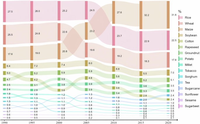
The temporal variation trends of crop harvest area in China. The height of the nodes represents the harvest area of crops, while the labelled text denotes the shares relative to the total harvest area for a certain year.
Figure 4 shows the spatiotemporal changes in harvest area for four crops (maize, rice, wheat, and soybean) from 1990 to 2020. The center of crop harvest is gradually shifting northward, with the Northeastern China emerging as a critical region for agricultural production. The maize cultivation is concentrated in the Northern and Northeastern China (Fig. 4a). There has been a steady increase in the area under maize cultivation since 1900, with a particularly accelerated pace after 2005. In particular, the most significant maize expansion occurred in the Northeastern China, resulting in a shift of the center by approximately 214 kilometers to the northeast. Rice cultivation is concentrated mainly in the middle and lower reaches of the Yangtze River, followed by the Northeastern China (Fig. 4b). Between 1990 and 2000, a significant decline was observed in the Zhejiang and Jiangsu Provinces. In contrast, there was a notable expansion in the Northeastern China as well, resulting in a shift of about 344 kilometers to the northeast. The wheat cultivation is clustered in northern China, including Henan, Hebei and Shandong Provinces (Fig. 4c). As wheat production has become increasingly concentrated in the Huang-Huai-Hai Plain, the center of wheat production has shifted only 44 kilometers. Soybean cultivation is mainly concentrated in the Northeastern and Northern China (Fig. 4d). Heilongjiang and Inner Mongolia Provinces have been constantly extending their soybean area, resulting in a shift of the center by about 354 km to the northeast. The spatial distribution of non-staple crops exhibits significant heterogeneity, yet their primary cultivation centers are spatiotemporally stable (Fig. S9). For instance, rapeseed is predominantly concentrated in Central China (e.g., Hubei and Hunan provinces), whereas peanuts, millet, sunflower seeds, sorghum, and sesame are mainly cultivated in northern regions (e.g., Henan, Hebei, and Inner Mongolia). Furthermore, the primary harvest of potatoes, tea, sugarcane, and tobacco occurs in the southwestern provinces, including Yunnan, Guizhou, and Guangxi. Moreover, the primary production regions for cotton and sugar beet have shifted from North China to Xinjiang province.
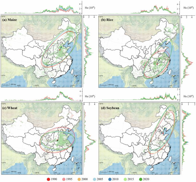
Spatiotemporal change of the crop harvest area in China. The distinct colors represent different years. The ellipses denote the standard deviation ellipses of crop harvest area distribution, while the dots indicate the centers of these ellipses. Profile graphs illustrating harvest area along both longitudinal and latitudinal directions are provided at the top and right side of the map. The background map is derived from the free open-source map dataset provided by Natural Earth (https://www.naturalearthdata.com).