Conceptual framework
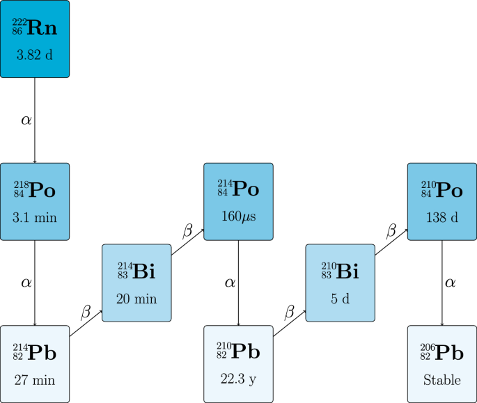
We speculate that there is an opportunity to estimate PMI using the relative abundance of radioactive decay products generated from naturally occurring (^{222}textrm{Rn}) and that is absorbed by living systems. More specifically, the inhalation of radon gas and its decay products is functionally universal on Earth, as (^{222}textrm{Rn}) is generated by uranium isotope-bearing minerals within the lithosphere and migrates via free-phase gas and water to the surface, where it enters the atmosphere of including indoor and outdoor air environments occupied by people20,21. Human populations are exposed to some amount of radon and radon decay products daily, which is typically measured in an indirect manner by evaluating the amount of alpha particle emissions per second (Bq) per cubic metre of air ((Bq/m^3))22. (^{222}textrm{Rn}) levels in outside air are typically measured in the 1-60 (Bq/m^3) range23,24,25, although can be (>100) (Bq/m^3) in exceptional cases26. Indoor air or subterranean air radon amounts can be anything from 10-100,000 (Bq/m^3), depending on building and region20. (^{222}textrm{Rn}) has a relatively short half-life of 3.8 days before undergoing a series of radioactive decays to form a series of very short lived ((t_{1/2}) = microseconds to minutes) isotopes of Po, Pb and Bi before becoming long-lived (^{210}textrm{Pb}) ((t_{1/2}) = 22.3 years), then (^{210}textrm{Bi}) ((t_{1/2}) = 5 days), (^{210}textrm{Po}) ((t_{1/2}) = 138 days), and finally stable (^{206}textrm{Pb}) (Figure 1).
Although exposure to some amount of gaseous (^{222}textrm{Rn}) and solid radon decay products is functionally universal, the specific amount of these radioisotopes inhaled by a person occurs at variable amounts across a lifetime depending on where they live, in what buildings they occupy, and behavioural factors such as occupation, tobacco use, diet and more27,28,29,30,31. It is important to understand that human exposure to radon and its decay products is a function of how much gaseous (^{222}textrm{Rn}) is constantly entering a given environment from geogenic sources, and also those radon-decay products that have equilibrated within the same environment via (^{222}textrm{Rn}) decay and attachment to particulates such as smoke or dust20. Both gaseous radon and the ‘attached fraction’ of radon decay products are inhaled and will be absorbed into living tissue via the lungs32,33,34. To a lesser extent, radon and its decay products can be ingested via drinking groundwater, eating certain foods such as (^{210}textrm{Pb})-rich lichen-eating wild game (e.g. caribou, elk, deer, moose), or tobacco smoking34,35,36. As all these routes of exposure demand that a person is alive, the deposition of (^{222}textrm{Rn}) and radon decay products within tissue is innately associated with life, whilst the cessation of breathing, drinking, and/or eating that occurs at death marks the end of incoming (^{222}textrm{Rn}) and radon decay products.
Careful measurement of the relative abundance of these decay products is now possible using recent advances in technology and so, for the first time, it is theoretically possible to use a radioisotopic decay of (^{222}textrm{Rn}) to evaluate PMI. Indeed, previous work by Ziad and colleagues37 explored the use of radon decay product ratio measurements to estimate time of death. Assumptions made during that investigation included constant radon exposure during life and an initial equilibrium value of (^{210}textrm{Pb}):(^{210}textrm{Po}) that complicates time of death estimation37; as these assumptions were undefined, they added uncertainties. We note that while the theoretical idea to measure (^{222}textrm{Rn}) decay products to estimate PMI is straightforward, its practical application is not. The accumulation of radon decay products in tissue is in the order of femtogram per gram (fg/g). Consequently, hypersensitive instruments are needed to measure isotope abundance (i.e. number of atoms) of radon decay products in biological tissues. If a low abundance measuring procedure is in place, as has been achieved for uranium or plutonium isotopes38, the next problem is to identify tissues that are helpful to measure within the context of a corpse, based how radon decay products are stored in the body. Current evidence suggests that, in addition to the lungs, keratinizing tissue (nails), adipose tissue (fat), and bone are all tissues where radon decay products have been empirically found to accumulate33,34. To develop and evaluate a theoretical model, we divided our work into two consecutive phases: the forward model and the actual Radon Time of Death Clock calculation. Our rationale was to use the radioactive decay equations under the assumption of a steady source of radon to generate data that could then be used to test the accuracy of the Radon Time of Death Clock. A critical component of the Radon Time of Death Clock developed here is the use of (1) relative numbers of isotopes and (2) two pairs of isotope abundance ratios. These input data enable a determination of the elapsed time since death to very high accuracy and is a key feature of this approach.
The forward model
For the forward model, we conceptualized a person who inhaled air containing an average of 100 (Bq/m^3) radon from birth to the time at which they died (time of death = (t_d)). The radon exposure assumption reflects the reality of radon in many nations including, for example, Canada where recent outcomes of national surveying found that the geometric mean, weighted level of radon in a residential building is 84.7 (Bq/m^3), with 42(%) of people experiencing levels of radon 100 (Bq/m^3) or more. For the forward model, we also assumed inhalation of radon and all radon decay products ceased entirely at the time of death, and that the numbers of (^{210}textrm{Pb}), (^{210}textrm{Bi}), and (^{210}textrm{Po}) atoms each began to decrease according to radioactive decay laws and their respective radioisotopic decay probabilities. At specific times after the discovery of the theoretical corpse by investigating authorities, we assumed the measurements of radon decay products in one or more tissues from the body could be performed (time of measurement = (t_m)), including the numbers of remaining atoms and isotope number ratios.
We suggest that two ratios that involve three radon decay isotopes ((^{210}textrm{Pb}), (^{210}textrm{Bi}), and (^{210}textrm{Po})) are of particular interest, as these isotopes have relatively longer half-lives; these ratios are: (r_1 = frac{^{210}textrm{Pb}}{^{210}textrm{Po}}) and (r_2 = frac{^{210}textrm{Pb}}{^{210}textrm{Bi}}). Starting with zero atoms for all the species of interest, and having a set of decay rates, we can obtain the ratios of the number of atoms at any time before or after death. The decay equations guarantee existing a unique set of ratios for any specific set ({t_d, t_m}),
$$begin{aligned} begin{aligned}&hbox {d}{N_{0}}{t} = A – lambda _0 N_{0},\&hbox {d}{N_{1}}{t} = lambda _0 N_{0} – lambda _1 N_{1},\&hbox {d}{N_{2}}{t} = lambda _1 N_{1} – lambda _2 N_{2},\&hbox {d}{N_{3}}{t} = lambda _2 N_{2} – lambda _3 N_{3}, end{aligned} end{aligned}$$
(1)
In this scenario, the value A (Bq) represents the constant activity level of radon in air, and ((lambda _0, N_{0})), ((lambda _1, N_{1})), ((lambda _2, N_{2})), ((lambda _3, N_{3})) denote decay constants and number of atoms for (^{222}textrm{Rn}), (^{210}textrm{Pb}), (^{210}textrm{Bi}) and (^{210}textrm{Po}), respectively. However, after death, the first equation follows:
$$begin{aligned} hbox {d}{N_{0}}{t} = – lambda _0 N_{0}, end{aligned}$$
(2)
In this scenario, the supply of radon to the body ceases, the (^{222}textrm{Rn}) atoms undergo decay and, since the person is no longer inhaling air, there is no source to replenish the (^{222}textrm{Rn}) atoms. Below are the solutions to the above equations before death:
$$begin{aligned} N_{1}(t)= frac{A lambda _0 (1- e^{-lambda _1 t})}{lambda _1}, end{aligned}$$
(3)
$$begin{aligned} N_{2}(t)= frac{A lambda _0 (lambda _1 (1-e^{-lambda _2 t})+lambda _2 (e^{-lambda _1 t}-1))}{(lambda _1-lambda _2) lambda _2}, end{aligned}$$
(4)
$$begin{aligned} begin{aligned} N3(t)= frac{A lambda _0 e^{-(lambda _1+lambda _2+lambda _3) t}}{(lambda _1-lambda _2) (lambda _1-lambda _3) (lambda _2-lambda _3) lambda _3}times&[(lambda _1^2 e^{lambda _1 t} (lambda _2 e^{lambda _2 t} (e^{lambda _3 t}-1)-lambda _3 e^{lambda _3 t} (e^{lambda _2 t}-1)) \&+lambda _1 e^{lambda _1 t} (lambda _3^2 e^{lambda _3 t} (e^{lambda _2 t}-1)-lambda _2^2 e^{lambda _2 t} (e^{lambda _3 t}-1))\&+lambda _2 (lambda _2-lambda _3) lambda _3 e^{(lambda _2+lambda _3) t} (e^{lambda _1 t}-1))]. end{aligned} end{aligned}$$
(5)
A Monte Carlo simulation was done where the age of the individual and the time that elapsed between death ((t_d)) and the measurement ((t_m)) were varied. Specifically, (t_{d}) varied between 20 and 40 years and (t_m) varied up to 20 days. The simulation was run 3,500 times to create multiple sets of (frac{^{210}textrm{Pb}}{^{210}textrm{Bi}}) and (frac{^{210}textrm{Pb}}{^{210}textrm{Po}}) isotope number ratios, with each pair having a known (t_{d}) and (t_{m}).
The (^{222}textrm{Rn}) main decay chain and daughter products. The half-life of each isotope is indicated. Only the dominant decay pathways are shown and low-probability branches (e.g., (^{218}textrm{Po}) to (^{218}textrm{At})) are omitted for clarity.
The radon time of death clock
We next used the data generated from Monte Carlo simulations as input quantities to the Radon Time of Death Clock, to test its theoretical accuracy, meaning how well outcomes predicted a known time of death. The calculation of the elapsed time for measuring the numbers of (^{210}textrm{Pb}), (^{210}textrm{Bi}), and (^{210}textrm{Po}) atoms ((t_{m})) was based only on the relative isotope number ratios. Thus, the input quantities to the Radon Time of Death Clock were the (r_1) and (r_2) ratios. Here, we assumed the individual was exposed to a constant level of radon over their lifetime. The model was implemented in Python 3.0 and employs the “brute force” method that involved calculating the function’s value at each point on a multidimensional grid to determine the function’s global minimum, and the Nelder-Mead minimization algorithm to calculate the elapsed times between death and measurement of isotopic composition.
The model solved the radioactive decay equations simultaneously for the two pairs of number ratios such that, although the radioactive decay probabilities for each radionuclide are different, the elapsed time for radioactive decays must be the same. Very importantly – as it would be impractical in the field – knowledge of the absolute radon exposure of the person at the time of death was not needed, as this quantity was cancelled out in the calculation since equations employed the relative number of isotopes (i.e. (^{210}textrm{Pb}) to (^{210}textrm{Bi}) and (^{210}textrm{Pb}) to (^{210}textrm{Po})). The use of two sets of the relative numbers of isotopes enabled the calculation of a unique answer. In the case of using a single isotope number ratio in the calculation (i.e. only (^{210}textrm{Pb}) to (^{210}textrm{Bi})), the result from the model was not unique. However, if both relative isotope number ratios were input to the model, then the result was constrained to a much narrower range of possible values for the time elapsed between death and measurement, where a solution to the equations is found.
Constant lifetime radon exposure
In the hypothetical scenario of constant radon exposure during a lifetime, we define a two-dimensional vector field, (vec {r} = vec {S}(t_d, t_m)), where (vec {r} = (r_1, r_2)). Vector field (vec {S}) can be evaluated based on decay equations for any valid set ({t_d, t_m}), either analytically or numerically. We consider evaluating vector field (vec {S}) at any given time set to be ‘solving the direct problem’ – i.e., solving the direct problem simulates a reality in which a person lived for a specific time with a constant radon exposure, died at (t_d), and the (r_1) and (r_2) ratios are measured at (t_d + t_m). The components of (vec {S}(t_d, t_m)) give us the ratio values in the ideal case of no uncertainty in the measurement results.
Assuming that there is a unique set of times, ({t_{d,T}, t_{m,T}}), which leads to a specific set of measured ratios, ({r_{1,T}, r_{2,T}}) (i.e. (vec {r}_T = (r_{1,T}, r_{2,T}) = vec {S}(t_{d, T}, t_{m, T}))) that we define ’solving the inverse problem’ as follows. The subscript T denotes the true value, which is presumed to be measured. Due to the absence of uncertainty, this true value should correspond to the value obtained from the forward model. When defining the scalar field,
$$begin{aligned} E_{vec {r}_T}(t_d, t_m) = left| vec {S}(t_d, t_m) – vec {r}_Tright| , end{aligned}$$
(6)
we suggest that there should be one single global minimum for (E_{vec {r}_T}) which happens at ((t_{d, T}, t_{m, T})). Hence, for a given set of valid ratios, (vec {r}_T), one can find the set of times, ({t_{d, T}, t_{m, T}}), that leads to the measured ratios, by minimizing the scalar field (E_{vec {r}_T}).
To test the accuracy of the model, we next calculated the elapsed time since death for the isotope pairs produced by the Monte Carlo simulations. The results are shown in Figure 2a, where the difference between actual and calculated elapsed measurement times (optimization error) are plotted as a function of the time that has elapsed since death. Outcomes demonstrate that the Radon Time of Death Clock could provide reliable results within just a two-week window after actual the death of the individual, and were remarkably precise with the average absolute error of 114 milliseconds. The consistency of the results was supported by a standard deviation of approximately 141 milliseconds. The error distribution arising from a scenario involving constant radon exposure and a single time measurement of two isotope pairs is shown in Figure 2b.
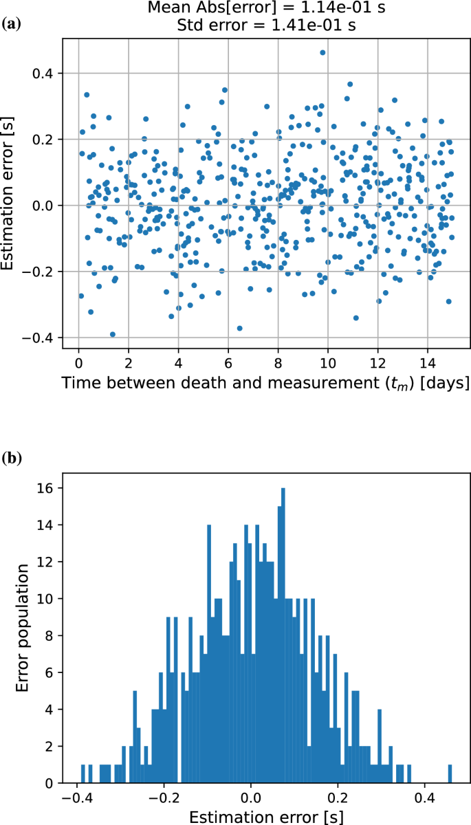
(a) Difference between the true and calculated elapsed time since death using the two pairs of isotope number ratios. Note that no uncertainty was assumed for the input quantities to the model. The RTDC could calculate the accurate time of death to within seconds. (b) Distribution of errors in post-mortem interval estimation under constant radon exposure conditions, showing Gaussian distribution pattern of discrepancy between predicted and actual time since death.
Accounting for variation in radon exposure across a lifetime
In reality, people are exposed to (^{222}textrm{Rn}) and solid radon decay products at a variable rate and at different levels across their lifespan20,21,28,39. Empirical evidence for ever changing radon exposure across a lifetime exists and has been demonstrated, with shifts in exposure caused by life events such as entering the workforce, changing profession, starting or stopping tobacco smoking, moving house, entering retirement, obtaining a radon reduction, and/or more systemic events such as implementation of pandemic emergency lockdown responses telecommuting, or nation wide building code changes27,28,29,30,31. So, to make the model more realistic, we next modeled a scenario where we assumed that the rate of radon exposure undergoes multiple changes during individual’s lifespan (albeit, for simplicity, each period of exposure was constant between jumps).
Similar to the case of constant exposure, we define the vector field (vec {r} = vec {S}_{f(t)}(t_d, t_m)), where f(t) is a piece-wise constant function of time that gives the overall rate of radon exposure activity over time. Note that the rate of radon exposure activity is defined only within the time between conception and death and that, after death, all relevant radionuclides will decay with no further input from parental (^{222}textrm{Rn}) and/or solid radon decay products. Therefore, all the discontinuities of f(t) should satisfy (0
$$begin{aligned} f(t) = {left{ begin{array}{ll} a_1 quad quad quad & ,0< t< t_1\ a_2 & ,t_1< t< t_2\ vdots \ a_N & ,t_{N-1}< t< t_N\ a_{N+1} & ,t_N< t< t_d\ 0 & ,t_d < t end{array}right. }, end{aligned}$$
(7)
Here, N is the number of jumps in the rate of radon exposure activity the person experiences, while (t_n in T_{jumps}) is the time of (n^{th}) jumps, and (a_j in jumps) is the constant value describing the rate of radon exposure activity between two successive jumps.
In an ideal scenario, solving the inverse problem would determine the set of parameters ({t_d, N, jumps, T_{jumps}, t_m}), in which N is the number of jumps, jumps, is the set of activity values between the jumps, and (T_{jumps}) is the set of times of jumps before (t_d), such that these lead to a set of ratios that match with the measured values in reality (or the outcome of (vec {S}_{f(t)}(t_d, t_m))). However, from a practical perspective, solving such a problem would far too computationally expensive to be helpful (i.e., impractical using regular computers, as the number of unknown parameters is large). It can be claimed that if there is any piece-wise constant function (tilde{f}(t) ne f(t)) and (tilde{t}_dne t_d) such that,
$$begin{aligned} vec {S}_{tilde{f}(t)}(tilde{t}_d, 0) simeq vec {S}_{f(t)}(t_d, 0), end{aligned}$$
(8)
Then will have the equation below for any (t_m):
$$begin{aligned} vec {S}_{tilde{f}(t)}(tilde{t}_d, t_m) simeq vec {S}_{f(t)}(t_d, t_m), end{aligned}$$
(9)
The implication of this is that the post-mortem evolution of these radioisotopic ratios is predicted to follow a similar pattern regardless of the lifespan or lifetime radon exposure of the person, meaning this readout of PMI is agnostic to inter-individual differences, and so is likely helpful to forensic investigators who need to ascertain PMI. To move forward with evaluation our model, we proceeded under the assumption that it is feasible to replicate the post-mortem characteristics of (r_1) and (r_2) from a scenario with the death occurring at time (t_d) and multiple fluctuations in the rate of radon exposure activity over the lifespan. We used a less complex scenario where death happens at a different time (t_d^prime) ((t_d ne t_d^prime)) and involves a single change in rate of radon exposure activity. Although this approach is an approximation and will not exactly mirror the reality of lifetime radon exposure, it is a reasonable estimation for a wide range of cases. To formulate the aforementioned approximation, we initially define a step-function g(t) as follows,
$$begin{aligned} g(t) = {left{ begin{array}{ll} a_1 quad quad quad & , 0< t< t_1\ a_2 & , t_1< t< t_d\ 0 & , t_d < t end{array}right. }. end{aligned}$$
(10)
Since we deal with the ratios, the absolute values of (a_1) and (a_2) do not affect the results directly, rather, the ratio (a = a_2/a_1) is what is important for us. So, we redefine the function g(t) to reduce the number of parameters,
$$begin{aligned} g(t) = {left{ begin{array}{ll} 1 quad quad quad & , 0< t< t_1\ a & , t_1< t< t_d\ 0 & , t_d < t end{array}right. }. end{aligned}$$
(11)
Now, with having (vec {r}_T = vec {S}_{f(t)}(t_{d, T}, t_{m, T})), we define the scalar field,
$$begin{aligned} E_{vec {r}_T}(t_d, t_m, t_1, a) = left| vec {S}_{g(t)}(t_d, t_m) – vec {r}_Tright| . end{aligned}$$
(12)
Similar to the case of constant activity, by minimizing the scalar field (E_{vec {r}_T}), we can obtain the set of parameters that result in the ratios of interest, and those parameters include (t_m).
Measurement of radioisotope ratios at multiple times postmortem
The theoretical approach we have described so far yields generally satisfactory outcomes. However, in certain instances, we observed that it can lead to very large uncertainty on (t_m) values. The discrepancy arises because the parameters ({t_d, t_m, t_1, a}) that result in (vec {r}_T) are not unique, and an example where the method fails is depicted in Figure 3.
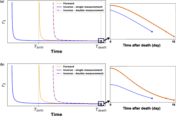
This figure demonstrates how minimization is used to estimate the time of death based on forward model data. A single postmortem measurement, which did not match accurately the true time of death, was also analyzed using double measurement approaches. Under lifetime-varying radon exposure, the minimization curve deviates from the forward model (true ratio curve) when using a single postmortem measurement. In contrast, the dashed line representing the double measurement approach closely matches the forward model. (a) shows the minimization result for isotope ratio (r_{1}(frac{^{210}textrm{Pb}}{^{210}textrm{Po}})) and (b) the minimization result for isotope ratio (r_{2}(frac{^{210}textrm{Pb}}{^{210}textrm{Bi}})).
In all cases, the resulting ratios match those obtained from the forward model simulation. However, there is a notable discrepancy in the estimation of (t_m). To address this issue, one approach we suggest is to incorporate radioisotope ratios with their rates of change (time derivative) into the analysis. As an approximation of the time derivative, a second measurement of ratios can be introduced into the scenario. The first measurement takes place at (t_{1,T} = t_{d,T} + t_{m,T}), and the second measurement at the time (t_{2,T} = t_{d,T} + t_{m,T} + t_text {step}). The outcomes are denoted as (vec {r}_{1,T} = (r_{1,1,T}, r_{2,1,T})) for the first measurement and (vec {r}_{2,T} = (r_{1,2,T}, r_{2,2,T})) for the second one.
$$begin{aligned}&vec {r}_{1,T} = vec {S}_{f(t)}(t_{d, T}, t_{m, T}), end{aligned}$$
(13)
$$begin{aligned}&vec {r}_{2,T} = vec {S}_{f(t)}(t_{d, T}, t_{m, T} + t_text {step}). end{aligned}$$
(14)
Then we define the scalar field that should be minimized as,
$$begin{aligned} begin{aligned} E_{vec {r}_{1,T},vec {r}_{2,T}}(t_d, t_m, t_1, a) =&left| vec {S}_{g(t)}(t_d, t_m) – vec {r}_{1,T}right| + left| vec {S}_{g(t)}(t_d, t_m+t_text {step}) – vec {r}_{2,T}right| . end{aligned} end{aligned}$$
(15)
The error distribution for a model with varying radon exposure and two measurements of two isotope pairs that are separated in time is in Figure 4. Since no measurement of isotopic composition is free from uncertainty, a preliminary study was carried out to explore the sensitivity of the Radon Time of Death Clock to measurement errors. An initial run introduced random error to the the (r_1) and (r_2) isotope number ratios and the model calculations were repeated using a relative standard deviation of 0.01 percent in the ratios. Under these conditions, the uncertainty in the elapsed time calculation increased to approximately 1 day. To explore the theoretical limit of the model’s temporal resolution, calculations were repeated assuming a relative uncertainty of 0.01(%) in the isotope ratios. While this level of precision is not currently achievable using standard detection techniques, it serves as an upper-bound scenario to evaluate model behavior under idealized conditions, such as might become accessible through future advances in measurement technology.
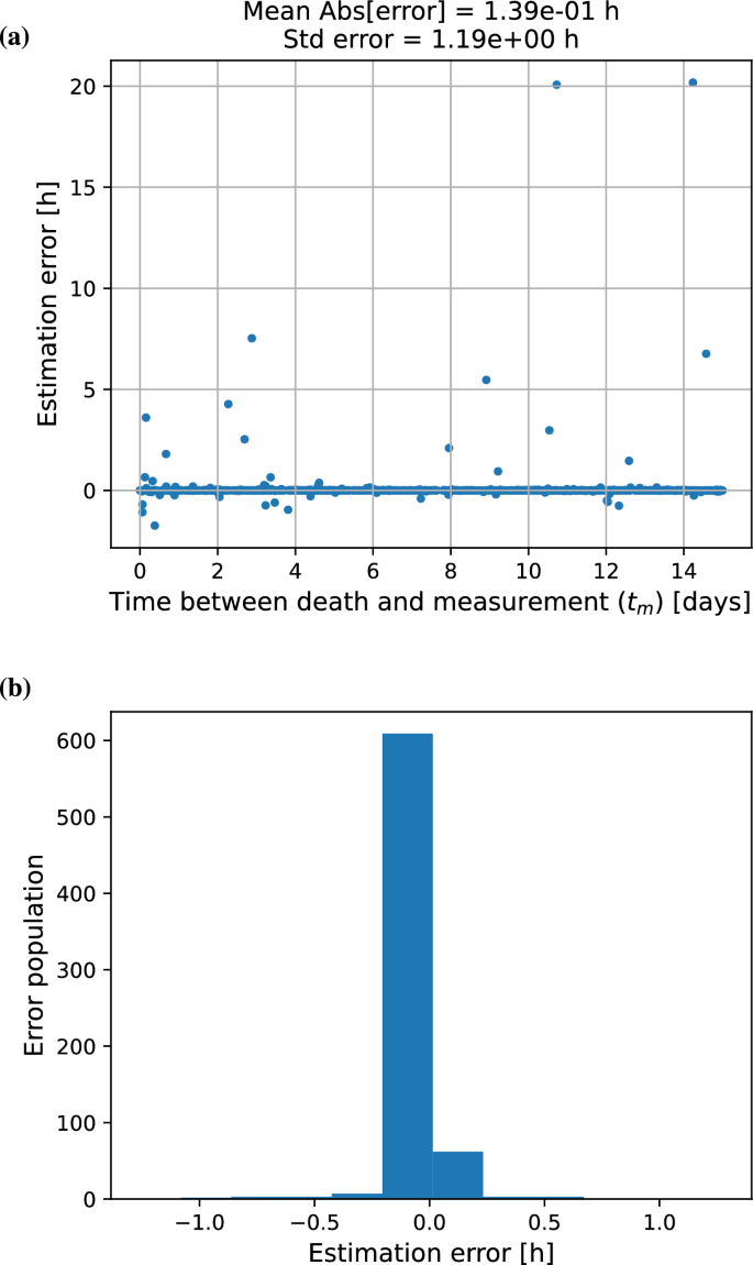
(a) Difference between the true and calculated elapsed time since death using two pairs of isotope ratios. The study employed a double measurement approach, where two pairs of isotopes were measured twice at separate time intervals. Note that no uncertainty was assumed for the input quantities to the model. The RTDC could calculate the accurate time of death to within 10 minutes. (b) Distribution of optimization errors in post-mortem interval estimation under varying radon exposure conditions, showing Gaussian distribution pattern of discrepancy between predicted and actual time since death.