Araghchi says ready and ‘waiting’ for US invasion; Tehran strike sparks Bahrain refinery blaze
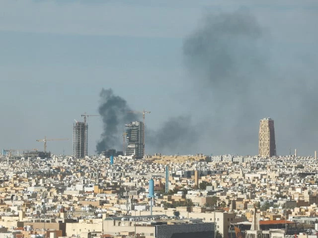
Smoke rises above the city skyline in Riyadh, amid the US-Israeli conflict with Iran. Photo: Reuters
…
Araghchi says ready and ‘waiting’ for US invasion; Tehran strike sparks Bahrain refinery blaze
Smoke rises above the city skyline in Riyadh, amid the US-Israeli conflict with Iran. Photo: Reuters
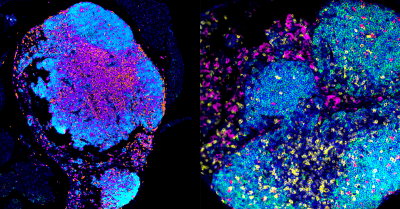
Newswise — Researchers at the University of California San Diego and collaborators have discovered a new way to help the immune system fight ovarian cancer by changing how tumors communicate with nearby immune cells. The…
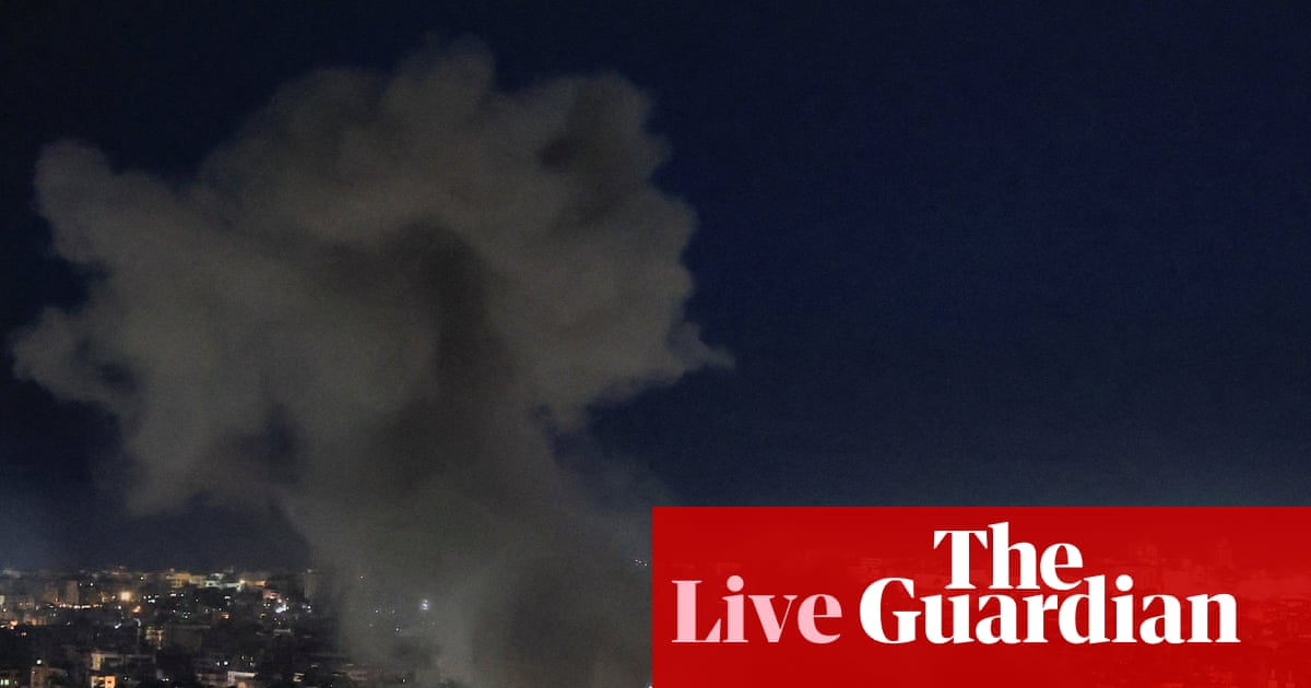
One beneficiary of the chaos in the Persian Gulf appears to be Russia, since the US treasury secretary, Scott Bessent, just announced that the US has issued a…

Over the years, a lot of scam WhatsApp mass messages claimed the service would imminently become paid. That hasn’t happened, obviously, and still won’t – the core service will remain free. However, WhatsApp is now rumored to be soon…

All three…
Abrupt reductions in global health funding for TB could impose tens of billions of dollars in additional costs on affected households in low- and middle-income countries (LMICs), with the heaviest burden falling on the poorest…

Rounding off the night, a group of Impressionist pictures demonstrated the movement’s enduring appeal. Claude Monet’s verdant painting of a Parisian urban oasis Le Parc Monceau (1878) made £6,760,000; Edgar Degas’s pastel of a nude bather

Are you experienced? This past week, Apple released the new iPhone 17e, M4 iPad Pro, new MacBooks, and more, and held its Apple Experience event. We’re covering it all on this episode of the Macworld Podcast.
This is episode…
One beneficiary of the chaos in the Persian Gulf appears to be Russia, since the US treasury secretary, Scott Bessent, just announced that the US has issued a…