- PM Sharif launches residential sector investment drive samaa tv
- Govt working on developing ‘mortgage finance’ ecosystem for housing, PM told Dawn
- Plan to revive real estate sector with Gulf investment amid war Dunya News
- Pakistan unveils new…
Author: admin
-
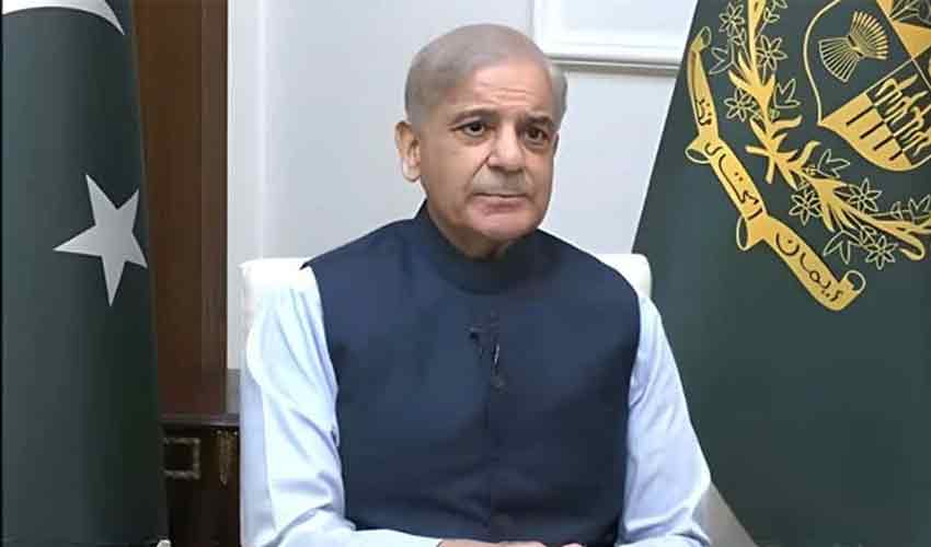
PM Sharif launches residential sector investment drive – samaa tv
-
Mega Discounts on Top-Rated Lenovo PCs and Tablets at Amazon's Big Spring Sale – PCMag
- Mega Discounts on Top-Rated Lenovo PCs and Tablets at Amazon’s Big Spring Sale PCMag
- Best Buy Slashes Lenovo 15.6-Inch IdeaPad to an All-Time Low, Rivaling Amazon’s Spring Sale Laptop Deals Gizmodo
- 4 laptop deals worth checking start at…
Continue Reading
-

Security guard at center of Chappell Roan controversy breaks silence
Security guard Pascal Duvier, most recently infamous for allegedly scolding 11-year-old Ada Law at a hotel in São Paulo, is clearing the air.
Duvier issued a statement on Instagram on Wednesday night following four days of back-and-forth social…
Continue Reading
-
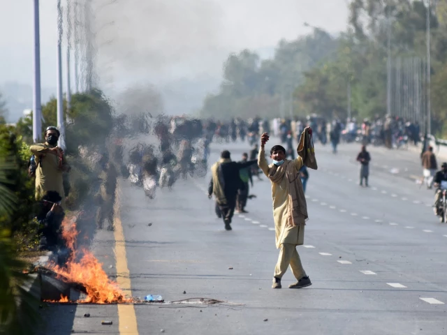
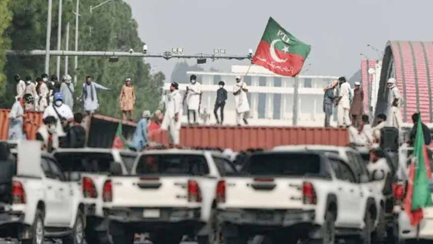
ATC extends interim bail for PTI leaders in Nov 26 protest cases
Islamabad court bars arrests until May 21 in over 230 cases linked to Sangjani rally and demonstrations
Supporters of the former Pakistani Prime Minister Imran Khan’s party, Pakistan Tehreek-e-Insaf (PTI), attend a protest demanding the release of…
Continue Reading
-

Dhurandhar: The Revenge crosses ₹1,000 crore worldwide, equals Pushpa 2 record in just 7 days
Aditya Dhar’s Dhurandhar: The Revenge joins the Rs 1,000 crore club in just 7 days. Check out the latest box office records and collection updates here.
Dhurandhar 2 Mumbai: Dhurandhar:…
Continue Reading
-
Pakistan minister hits out at Imran Khan’s sons over UN remarks, GSP+ debate – Arab News
- Pakistan minister hits out at Imran Khan’s sons over UN remarks, GSP+ debate Arab News
- Imran’s son Kasim raises father’s case at UNHRC, decries his treatment in jail Dawn
- Kasim urges UNHRC intervention to end Imran’s persecution, detention…
Continue Reading
-
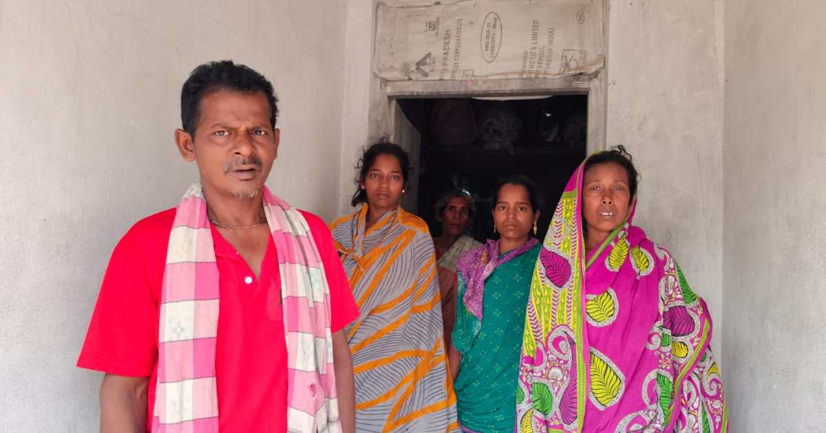
Deaths and debts: Missiles in Gulf shake millions of South Asian families | US-Israel war on Iran
A week into the United States-Israeli war on Iran, and Iran’s attacks on its Gulf neighbours, Jaya Khuntia spoke – as he often did – to his Doha-based son Kuna on the phone.
It was March 6, about 10pm, and Khuntia and the family were…
Continue Reading
-
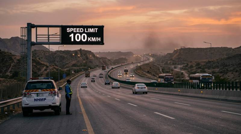
Reduced speed limits enforced on motorways, highways nationwide
The National Highways and Motorway Police has enforced reduced speed limits on motorways and national highways across Pakistan as part of the government’s fuel conservation and energy efficiency measures.
The move, implemented on the…
Continue Reading
-
ATC bars arrest of PTI leaders until May 21
Summary
The court extended interim bail in more than 230 cases involving the PTI leaders.…Continue Reading
-

Bristol balloon pilot on the verge of breaking world record
A balloon pilot is on the verge of breaking a world record for taking off in the highest number of countries around the world.
Allie Dunnington, from Bristol, has launched balloons in more countries than any other female pilot and is now on a…
Continue Reading