Category: 3. Business

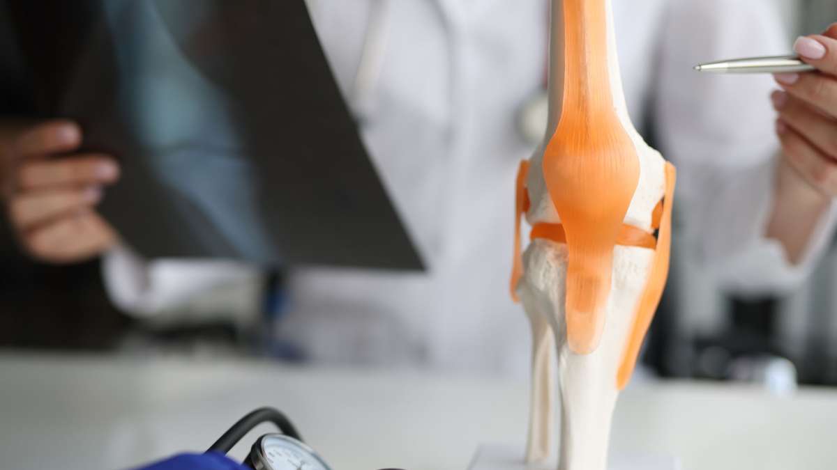
Suzuki Pakistan has announced a massive discount for a limited time on one of its popular models.

In a post on its social media handles, the company has announced a limited time offer of Rs. 450,000 cash bonus or discount on purchase of Suzuki Every.

The company has also outlined certain conditions for the offer that include:

• Offer is valid for a limited time only
• Applicable on Suzuki Every VX model only
• Offer may vary by dealership or stock availability.
• Suzuki Pakistan reserves the right to modify or cancel the offer at any time without prior notice.

For further details you can visit the Suzuki Pakistan website or your nearest dealership.

I moved to Stockholm from London for work a decade ago. As a newcomer with a passion for nature, I remember being eager to soak up the region’s archipelago of 30,000 islands and rocky outposts. But I was overwhelmed by complex public ferry timetables to dozens of places ending in the letter “ö” (the Swedish word for island) and uninterested in pricey cruise boats packed with tour groups.

Then a former flatmate recommended Nynäshamn, which is on the mainland but embodies much of the nature and spirit of Stockholm’s archipelago. It’s home to a tasteful waterfront of colourfully painted bars and restaurants and a harbour packed with boats every summer, from simple dinghies to luxury yachts. Beyond, you can look across a clean, calm stretch of Baltic Sea, towards the island of Bedarön, flanked by pine trees and a smattering of dark red detached houses.

Mention Nynäshamn to Stockholmers and most will probably describe it as the port you pass through to catch the four-hour ferry to Gotland – Sweden’s largest island – or an overnight cruise to Gdańsk in Poland. But for international tourists (or new Swedish residents, as I was), it is an entry-level coastal destination where you can get a taste of the city’s island life without the complex logistics.

Nynäshamn is on the commuter rail line from central Stockholm, and reachable in an hour. A one-way journey costs 43 kroner (£3.30), or it’s free if you have a valid monthly or weekly pass for the capital’s public transport system. For a little more adventure, it takes a further 30 minutes to reach Nåttarö, the closest island accessible by a public ferry service (£8 each way).

My first destination in Nynäshamn is Trehörningen, an island suburb accessible by bridge, and just a 30-minute stroll from the train station. The route takes in a mishmash of glassy new-build apartments, low-rise 1960s rent-controlled flats and mansions with manicured gardens. Nynäshamn doesn’t have the swagger of swankier seaside towns in the region, such as Sandhamn or Saltsjöbaden, but it offers a slice of real-life small town Sweden far removed from the well-trodden tourist itineraries that typically lead to Stockholm’s medieval Old Town or isolated rural retreats.

“It’s very good for my health,” says Hans “Hasse” Larsson, a smiley 73-year-old former truck driver who moved to Nynäshamn from Stockholm 16 years ago. He enjoys the clean air and quiet lifestyle, and describes a stronger sense of community compared with the somewhat stiffer Swedish capital. “Even if you don’t know people very well, you’ll say ‘hej’!” he laughs.

Sweden isn’t a budget destination, but thanks to a favourable exchange rate, prices aren’t extortionate compared with those in popular British seaside destinations I’ve visited, such as Brighton or St Ives. On Trehörningen island, it costs from just over £100 a night to rent a compact wooden cottage for two from Oskarsgatan 12 B&B. A breakfast buffet and spa entry package at the nearby Nynäs Havsbad hotel works out at around £45. The spa’s pavilion is a reconstruction of an art nouveau-inspired resort built in 1906, complete with an outdoor hot tub, a sauna and panoramic views. The hotel complex includes original buildings from the early 20th century, when it was a base for sailors during the 1912 Stockholm Olympic Games.

From here, it’s a short walk to Strandvägen, a French riviera-inspired waterfront road built for spectators of sailing. As locals will proudly tell you, it is the only place in the Stockholm archipelago region where you can see the horizon from the mainland. The scenic route winds towards Lövhagen, a wooded area offering shady trails and picnic tables. There are rocky swimming coves too – although, with average outdoor temperatures of 18C in July and August, the chilly waters won’t be to everyone’s taste.

For walkers, Nynäshamn is also a gateway to Sörmlandsleden, a system of hiking trails covering around 620 miles in total and clearly marked with orange arrows and painted tree markers. Section 5:1 from Nynäshamn passes through mossy forests and grassy farmland to the village of Osmö, where you can catch a train back to Nynäshamn or continue another nine miles to Hemfosa, snaking past Lake Muskan’s glistening waters.

Back at Nynäshamn’s main harbour, the restaurants are filling up with tourists hungry for lunch. The most famous spot is Nynäs Rökeri, a smokehouse dating back almost 40 years, where a platter of smoked salmon, seafood and potato salad costs less than £20. The adjacent delicatessen stocks fresh fish and classic Swedish treats, from cheesy västerbotten pie to crispbreads and lingonberry jam. A nearby courtyard is shared with customers visiting the ice-cream store Lejonet & Björnen, a small cafe and a gift shop.

The sweet smell of cinnamon wafts in the air and I spot the familiar logo of Skeppsbro Bageri, an award-winning Stockholm bakery that has a food truck parked on the waterfront, packed with fresh bread, buns and pastries. “I like it here,” says Emelie Elison, the 24-year-old student who is working in the van for her third summer in a row. “There are a lot of people and there’s always something happening.”

Sweden’s cities empty out in July, as locals flock to the coast to spend the summer in wooden holiday cottages. There are more than 600,000 of these holiday homes, known as fritidshus, which are often passed down through generations; almost half of children with at least one Swedish parent have access to one. They also have plenty of time to enjoy them – most Swedish employees are entitled to four consecutive weeks off each summer.

After a grey morning, the sun comes out as I join the ferry queue for Nåttarö. Many around me are armed with bags of groceries, backpacks and even suitcases, intending to stay at least a week. But one sporty-looking couple, carrying only tiny running backpacks, tell me they are fellow day-trippers from Stockholm, planning to run a six-mile loop of the Stockholm Archipelago Trail, a newly marked hiking and trail-running route stretching 167 miles across 20 islands.

Most tourists visiting Nåttarö take things at a slower pace. It’s a small, car-free island with one simple convenience store and two restaurants by the harbour. The main draws are the pine-lined walking trails, rocky clifftops and sandy beaches. There are 50 wooden cabins for hire (sleeping up to six people, £90 a night). The campsite is priced at less than £5 a night, including access to pristine showers, compost toilets and dishwashing facilities. Wild camping is allowed too, thanks to allemansrätten, Sweden’s right to roam policy.

I take a 1¼-mile trail to Skarsand, a small beach in the north-east of the island. I have fond memories of celebrating a friend’s 40th birthday here a couple of years ago, when we camped with friends and their kids, cooking dinner on the beach’s public grill. Today, despite being peak holiday season, I have it all to myself, save for some passing hikers.

The sunny afternoon passes quickly, and a couple of hours later I’m back on the ferry for Nynäshamn. The Stockholm pair have made it too, having successfully completed their run. They are eagerly awaiting a pizza reward at Maggan’s, another popular restaurant in Nynäshamn’s harbour, and tell me they’ve squeezed clean T-shirts into their backpacks to change into. I’m planning a sunny evening drink on the waterfront too. Tomorrow I’ll be at my desk, catching up on emails – and researching my next coastal adventure.

Microgrids (MGs), as defined by IEEE Std 2030.7™-2017, are self-sustaining energy systems capable of autonomous operation or functioning in grid-connected mode. These systems can seamlessly connect to and disconnect from the main power grid to exchange power, provide ancillary services, support grid stability, and participate in energy markets as needed. MGs are broadly classified as grid-connected or off-grid (islanded) and can be configured in AC, DC, or hybrid AC/DC modes, depending on the design objectives and operational requirements¹⁹.

To align with the Energy Trilemma (ET) framework, this study evaluates three key components:

• Energy Security: Represented by Loss of Power Supply Probability (LPSP), Voltage Deviation Index (VDI), and active power losses.

• Energy Access: Quantified using the Levelized Cost of Energy (LCOE).

• Environmental Sustainability: Assessed based on CO₂ emissions.

LPSP measures the fraction of the total energy demand that remains unmet due to system constraints within a given period. A lower LPSP indicates improved reliability and robustness of the microgrid. VDI quantifies voltage stability by evaluating deviations from nominal bus voltages, which is crucial for maintaining power quality and preventing system instability. Active power losses are analyzed to determine the overall efficiency of power transmission within the microgrid.

Recent years have seen a proliferation of advanced metaheuristic and AI-driven approaches for microgrid optimization. The Slime Mould Algorithm (SMA) was introduced in 2020¹⁴ and demonstrated superior global search and multi-objective capabilities for power system applications. Studies in 2023^15,17 benchmarked SMA against PSO, GA, and SSA, reporting higher power loss reduction and better computational efficiency in hybrid microgrid scenarios. Other work highlighted the scalability of SMA for larger distribution networks²⁰, and explored parameter adaptation for further runtime improvements^21,18.

In addition, recent studies have expanded the literature landscape: an AI-based approach for the optimal placement of electric vehicle charging stations (EVCS) and distributed generation (DG) demonstrated significant power loss minimization and voltage profile enhancement⁷. Adaptive particle swarm optimization methods have been proposed for allocating plug-in EV charging stations with integrated solar-powered DG, addressing both technical and economic performance¹⁰. A novel hybrid metaheuristic for optimal allocation of DG and capacitors showed marked improvements in system efficiency and power quality¹¹. A hybrid slime mould and salp swarm algorithm further validated the advantages of hybrid metaheuristics in microgrid planning¹². Finally, an improved SMA was applied for optimal scheduling of grid-connected microgrids with hybrid energy storage systems, reinforcing the applicability and robustness of SMA in complex, real-world scenarios^22,23.

Comparative studies have shown that while PSO and GA remain popular, their performance is often limited by premature convergence and high computational requirements, respectively. SSA offers improved convergence but may still lag behind SMA in multi-objective scenarios. HOMER, widely used for techno-economic microgrid analysis, is less effective for large-scale, multi-objective optimization and lacks the flexibility of metaheuristic algorithms as shown in Table 1.

Recent works have also explored the leading metaheuristic algorithms and simulation tools for microgrid optimization, revealing notable differences in their effectiveness across key performance metrics. The Slime Mould Algorithm (SMA) consistently demonstrates high power loss reduction—outperforming traditional approaches such as Particle Swarm Optimization (PSO) and Genetic Algorithm (GA) by 12–15%—while also achieving fast convergence and low iteration counts. SMA’s scalability is excellent, exhibiting linear runtime scaling even as network size increases, and its robust design enables comprehensive handling of technical, economic, and environmental objectives aligned with the energy trilemma framework^7,23,12.

In contrast, PSO and GA offer only moderate power loss reduction; PSO is prone to premature convergence and stagnation, whereas GA is hindered by high computational burden and slow convergence, particularly in larger or more complex networks^10,11. The Salp Swarm Algorithm (SSA) provides improvements over PSO and GA, especially in terms of convergence speed and scalability, but generally remains less effective than SMA for multi-objective optimization¹². HOMER, while widely used as a benchmark simulation tool, is efficient for small systems but lacks scalability and flexibility for large-scale or multi-objective microgrid optimization, focusing primarily on techno-economic assessments^15,20.

Overall, the evidence from recent literature underscores the superiority of SMA and highlights the growing importance of advanced metaheuristics for addressing the complex, multi-dimensional challenges of modern microgrid planning and operation.

System modeling and constraints

The Slime Mould Algorithm (SMA) was selected for this study due to its superior global search capability and adaptability in multi-objective optimization of complex power systems, as established in recent literature^14,20. The population size for SMA was set to 33, corresponding to the number of buses in the IEEE 33-bus test system, which ensures adequate solution diversity and effective exploration of the search space for optimal distributed energy resource (DER) placement; this choice was validated through preliminary runs and aligns with best practices reported^24,18. Other algorithmic parameters, including the maximum number of iterations (typically 100–200), inertia weights, and adaptive coefficients, were selected based on recommendations from the literature and fine-tuned to balance convergence speed and solution quality.

A sensitivity analysis was performed for DER sizing, particularly for solar distributed generation (DG), where the capacity was varied from 2,300 kW to 2,500 kW in 50 kW increments. The results indicated that increasing solar DG capacity from 2,300 kW to 2,400 kW reduced active power losses by approximately 3.5%, but further increases offered diminishing returns and, in some cases, led to over generation and curtailment, confirming that the SMA-optimized sizes provided the best trade-off among technical, economic, and environmental objectives, consistent with findings in^15,17.

Regarding computational complexity, SMA achieved convergence for optimal solar DG placement in 97 iterations with an average runtime of 8.2 min per optimization run, outperforming Particle Swarm Optimization (PSO), which required about 130 iterations (12.7 min), and Genetic Algorithm (GA), which needed 155 iterations (16.4 min) for comparable solution quality, corroborating the efficiency advantages reported in^14,20. All simulations were conducted in MATLAB R2023b on a standard workstation equipped with an Intel Core i5 processor (10th Gen, 2.4 GHz), 16 GB RAM, and Windows 11 OS, which was sufficient for the IEEE 33-bus system and allowed each full optimization run to complete in under 30 min; for larger networks, SMA’s runtime scales linearly with network size but remains tractable on similar hardware, as demonstrated in^25,26.

No specialized hardware such as GPU acceleration was required, making the approach practical for real-world engineering applications. The proposed Distributed Energy Resources (DERs) and their corresponding modeling parameters are detailed in Table 2. The microgrid configuration includes solar photovoltaic (PV) panels, wind turbines (WT), diesel generators (DGen), battery energy storage systems (BESS), and electric vehicle batteries (EVBat). Each energy source is modeled based on its rated capacity, operational constraints, and dispatch characteristics, ensuring optimal energy management and integration.

The modelling framework incorporates:

• Renewable Energy Generation Constraints: Solar PV and wind turbines exhibit variability, necessitating complementary storage solutions such as BESS and EV_Bat to enhance system stability.

• Backup Power Sources: Diesel generators provide reliability during low renewable generation periods.

• EV Battery Storage Integration: EV_Bats function as both loads and energy storage units, enabling vehicle-to-grid (V2G) operations, peak shaving, and frequency regulation.

• Operational and Economic Constraints: The optimization framework ensures that energy generation meets demand while minimizing costs and emissions.

The proposed hybrid microgrid

This study proposes an optimal topology and placement strategy for a Hybrid Battery-supported Microgrid (HBMG) within a radial distribution network. The primary objective is to minimize active power losses, thereby enhancing the voltage profile, reducing the levelized cost of energy (LCOE), and mitigating greenhouse gas (GHG) emissions. The proposed hybrid system integrates solar photovoltaics (PV), wind turbines (WT), a diesel generator (D_Gen), battery energy storage systems (BESS), and electric vehicle batteries (EV_Bat). The P/W/D/B/E configuration is designed to reliably supply electricity to meet the given load demand while also enabling surplus power injection into the grid when feasible^27,28,29,14. Figure 1 illustrates the schematic layout of the proposed HBMG model.

The system’s ideal integration location is optimally determined to minimize power losses and the cost of electricity generation in addition to CO₂ emission mitigation.

The proposed adopted network

Microgrids (MGs), as defined by IEEE Std 2030.7™-2017, are self-sustaining energy systems capable of autonomous operation or functioning in grid-connected mode. These systems can seamlessly connect to and disconnect from the main power grid to exchange power, provide ancillary services, support grid stability, and participate in energy markets as needed. MGs are broadly classified as grid-connected or off-grid (islanded) and can be configured in AC, DC, or hybrid AC/DC modes, depending on the design objectives and operational requirements.

To align with the Energy Trilemma (ET) framework, this study evaluates three key components: Energy Security: Represented by Loss of Power Supply Probability (LPSP), Voltage Deviation Index (VDI), and active power losses. Energy Access: Quantified using the Levelized Cost of Energy (LCOE). Environmental Sustainability: Assessed based on CO₂ emissions.

Technical details on HBMG configuration

The hybrid battery-supported microgrid (HBMG) configuration consists of distributed energy resources (DERs) such as photovoltaic (PV) systems, wind turbines (WT), diesel generators (DGen), battery energy storage systems (BESS), and electric vehicle batteries (EVBat). The optimal selection, sizing, and placement of these components are critical to improving system reliability and efficiency.

The proposed HBMG will be investigated using IEEE 33 bus standards distribution network nodes shown in Fig. 2. The IEEE 33-bus standard was adopted because of interoperability with both commercial and residential loads and moderate number of buses. In a similar advantage the networks is a balanced network at 12.66 kV and over 85% of loads are residential³⁰.

The network has 32 sections and total apparent power 4369.35 kW as seen in Fig. 2. The number of nodes is used as the population size during the optimization modelling process and the optimal bus location for DG integration was obtained based on the SMA convergence. The active, reactive and the apparent power of the IEEE 33-bus network is as shown in Table 3.

Slime mould algorithm overview

The study of slime mould algorithm (SMA) was first presented by³² as a bio-inspired metaheuristic algorithm. It simulates the morphological changes and behaviour of slime in foraging. The algorithm was bench-marked with thirty-three (33) algorithms under four (4) famous design problems and found to be superior in performance¹⁸. After this successful outcome, many studies have adopted the techniques to solve different single and multi-objective optimization challenges^18,33,34,35.

a. Initialization.

The mathematical formulation of the Slime Mould Algorithm (SMA), including initialization, position updating, and fitness evaluation, is adopted from the original work in¹⁴, with further enhancements and parameter tuning strategies incorporated from recent studies in^18,17. To capture the food approaching behaviour of the SMA or imitate the higher contraction approach of the SMA is shown mathematically in Eq. (1),

The position update equation for SMA is given as:

where (:a) and (:S) are adaptive parameters, as detailed in [Li et al., 2020,^1];

where(:overrightarrow{:vb}:) is a parameter which ranges from (:left[-a,aright]), (:overrightarrow{vc}) is a decreasing parameter which reduces from one to zero. (::t:)denotes the present iteration, (:overrightarrow{:{X}_{b}}:)is the possible location with the highest odour concentration, (::overrightarrow{X}:)is the present position of slime mould, (:overrightarrow{{X}_{A}}) and (:overrightarrow{{X}_{B}}) are two distinct locations randomly chosen from the swarm population, and symbol r is use to indicate the random values within the boundary of [0,1], while (:overrightarrow{W}) is the weight of slime mould. Whereas the population parameter (:p:)is defined by Eq. (3):

where (:i:varepsilon::text{1,2},dots:,n), (:Sleft(iright)) indicates the fitness of (:overrightarrow{X}), (:DF) denotes the best fitness recorded in the whole iterations. The parameter (:overrightarrow{vb}) ranges from -a to a as seen in Eq. (4) and the values of a are defined by Eq. (4)

where the maximum iteration is indicated by t_max.

The formula for weight of the slime (:overrightarrow{W}) and smellIndex are given in Eqs. (5) and (6):

In this context, the symbol S(i) indicates the one-half of the population size. bf shows the best fitness achieved in the present iteration, wF represents the less significant fitness value attained in the current iteration, finally (:SmellIndex) indicates the ranges of fitness values obtained in ascending order, specifically within the context of minimum value problem.

b. Updates stage.

The expressed formula for food wrapping and updating the position of the slime is given in Eq. (7):

where (:LB) and (:UB) indicates the lower and the upper intervals of the searching range, (:rand:)and (:r:) shows the non-linear value within [0,1] generated as a function of z and p respectively.

c. Oscillation stage.

The food grabble imitations shows ranges of (:overrightarrow{vb}:)moves non- linearly between [− a, a] and slowly settles down to zero as the number of iterations increases. While the parameter of (vc) moves between [− 1,1] and approaches to zero subsequently.

An appeal has been launched to try to get permission to build a new solar farm after a decision was not issued by a council in time.

Wessex Solar Energy (WSE) wants to install 40,000 solar panels on farmland near Haddon, in Cambridgeshire.

Huntingdonshire District Council failed to make a decision within the allotted timeframe, and the project will now be referred to the government Planning Inspectorate.

However, the council has recommended officers oppose the development on grounds of the potential impact on nearby Sibson Aerodrome.

A report published ahead of a council meeting on 18 August states: “The application has failed to demonstrate that it would not materially harm the safe functioning of Sibson Aerodrome or private flying strips through adverse impacts of glint and glare, and the loss of land necessary to facilitate emergency landings.”

WSE said the Haddon Road Solar Park would be able to export up to 25 megawatts, providing energy for up to 7,600 households a year.

The project follows similar plans for a larger solar farm of 65,000 solar panels, which was blocked by the district council last year after more than 100 objections were received.

A planning inspector later upheld this decision at an appeal, concluding that the development would cause “significant harm” to the area.

WSE has said its latest proposals for a smaller solar farm address the concerns raised about the previous project, the Local Democracy Reporting Service said.

The company said it accepted the proposed solar farm would have some impact on the area, but measures were proposed to minimise this, including strengthening field boundaries and retaining hedges.

In the previous section the ANN and ML methodologies for the prediction of the speed of sound of DESs has been described and depicted in Figs. 1 and 2. In this section the ANN + GC and ML + GC approaches have been described separately.

ANN + GC method

The number of independent variables (input layer) plays a crucial role in ANN and ML methods⁶³. In Table 1, thermodynamic properties of DESs containing T_c, V_c, MW, and ω have been reported. In the case of ANN method, different input properties and different numbers of neurons in one and two hidden layers have been considered, because one hidden layer only does not lead to adequate results^64,65,66,67. The number of the hidden layer and neuron in the hidden layer and output are obtained using a trial and error algorithm. In this work the Levenberg–Marquardt algorithm^68,69 is used to optimize the aforementioned parameters. The results show that, one hidden layer containing 16 neurons and four input properties containing the critical volume (V_c), molecular weight (Mw), temperature, and acentric factor (ω) are the optimum values. As described in section “Theory and methodology”, 300 training and 115 testing data points of the speed of sound have been considered.

As mentioned in Eq. (7), the weight parameters between neurons in hidden layers are essential to develop the network. In Table 4 the weight parameters of neurons have been reported.

The optimum values of neurons in the hidden layer are evaluated using the average relative deviation percent (ARD%). When the optimum network architecture was determined, the input data of the ten DESs were fed to the network to predict their speed of sound. In Fig. 3 the flowchart of the proposed ANN model has been depicted.

As shown in Fig. 3, the model can predict the speed of sound of DESs using independent variables containing T, V_c, ω, and MW. The inputs containing V_c, and ω can be estimated using GC approaches^45,46. Experimental literature data is used as the training dataset for sound speed. An ANN with one hidden layer containing sixteen neurons is employed to develop the model. Four input variables can be fed into the saved file to generate predicted sound speed. Using the “saved network” and these four inputs, the sound speed of DESs can be accurately predicted. The complete MATLAB code, including all source files used in the programming, is provided in the Supplementary Material. The correlated and predicted results of the ANN + GC approach have been shown in Fig. 4.

Figure 4 shows that the ANN + GC approach can correlate the speed of sound of DESs over a wide range of temperatures, satisfactory. The ARD% and R² of the correlated speed of sound have been obtained 0.032% and 0.9988, respectively. Figure 4b shows the prediction of the speed of sound of ten DESs using the ANN + GC approach. The results are in good agreement with experimental data. Figure 5 shows a simultaneous comparison between the experimental data and ANN + GC data.

As shown in Fig. 5, the ANN + GC method can correlate the experimental data accurately. Distributions of the deviation points for the ANN + GC method are shown in Fig. 6.

As shown in Fig. 6, the deviations between the ANN + GC predictions and experimental data do not exceed 4 m/s. Error analysis indicates that the proposed network is suitable for engineering calculations. In this study, the predictive performance of the ANN + GC model was assessed using R², ARD%, SD, MAE, and RMSE metrics; see Table 5.

As shown in Table 5, the total ARD%, MAE, SD, RMSE, and R² values have been obtained 0.032%, 1.5656, 0.0549, 2.227, and 0.9988, respectively. The results of the ANN + GC approach show good agreement with experimental data. Models with high R² values nearing 1 and low values for ARD%, RMSE, MAE, and SD are considered more accurate in predicting the speed of sound. In this study, the ARD% for the training and testing phases of the ANN + GC model were 0.024% and 0.053%, respectively. The overall R² value approached unity at 0.9988. These results indicate that the ANN + GC model can accurately correlate the speed of sound in DESs across a wide temperature range. In the next section, the ML + GC model has been studied.

ML + GC method

Similar to the ANN + GC method, the inputs for the ML + GC model included V_c, ω, Mw, and T. Additionally, 300 training and 115 testing data points of the speed of sound were used to develop the machine learning approach. The statistical metrics for the CatBoost model are summarized in Table 6, which presents evaluations on the training and testing subsets (300 and 115 data points, respectively), as well as the complete dataset consisting of 415 points. In this study, the predictive performance of the models was assessed using R², ARD%, SD, MAE, and RMSE metrics. Comparing model predictions with experimental data across both training and testing datasets provides valuable insights into the models’ accuracy and generalization capability; see Table 6.

The greater the alignment between the predicted value and the experimental data, the higher the accuracy of the predictive model. In Figs. 7 and 8, the error distribution plot of the presented model vs the predicted speed of sound has been depicted. This visual representation demonstrates the robust agreement between the experimental data and the forecasts produced by the CatBoost ML method.

Figures 7 and 8 illustrate a strong correlation between the model-predicted data and the experimental data across both the training and testing datasets. These figures demonstrate a very close alignment between the model predictions and experimental points. In this research, graphical analysis complemented statistical methods to provide a more comprehensive evaluation of the models’ performance. These visual representations played a vital role in assessing the accuracy and reliability of the models. The percentage distribution of the relative error against the experimental values is presented in Fig. 7. In this type of error evaluation, relative error values are plotted against experimental output values. The closer the data points are to the zero-error line, the model is the more accurate. When the data points are scattered around the zero line, it indicates a significant difference between the predicted values and the experimental data, which proves the high error of the model. As a result, the proximity of the data points to the zero line for the ML + GC model indicates the high accuracy of this model. In Fig. 8, the cross-plot has been depicted. The cross-plot visually represents the comparison between predicted and experimental values. A closer alignment of data points with the unit slope line (Y = X) in the cross plot signifies higher accuracy and effectiveness of the model. The ML + GC model shows significant performance with most of the data points lying around the Y = X line. In the next section, a comparison between ANN + GC, ML + GC, and the correlation-based models has been investigated.

Comparison between ANN + GC, ML + GC, and the correlation-based models

The ANN + GC and ML + GC results have been compared to five correlation-based models^{24,70,71,72,73}. Singh and Singh proposed a correlation for speed of sound based on the surface tension and density⁷⁰. Hekayati and Esmaeilzadeh suggested a novel interrelationship between surface tension (σ), density (ρ), and speed of sound (u) of ILs⁷¹. Gardas and Coutinho proposed a relationship between surface tension (σ), density (ρ), and speed of sound (u) for imidazolium based ILs, covering wide ranges of temperature, 278.15–343.15 K⁷³. The aforementioned models are correlation-based. In Table 7 the ARD% of five correlation-based, ML + GC, and ANN + GC models have been reported and compared.

The average ARD% value of Peyrovedin et al.²⁴ model was obtained 5.67%. ARD% values of Haghbakhsh et al.’s model⁷², Hekayati and Esmaeilzadeh’s model⁷¹, and Gardas and Coutinho’s model⁷³ for 38 DESs have been obtained 9.52%, 9.38%, and 9.45%, respectively. The average ARD% value of Singh and Singh’s model⁷⁰ was obtained about 39%. They correlated the speed of sound of ILs using surface tension and density data. As shown in Table 7, the Peyrovedin et al.²⁴ model gives a lower ARD% value compared to other correlation-based models. The ANN + GC and the ML + GC models give lower error values compared to correlation-based models. The ARD% of the ANN + GC model is slightly lower than the ML + GC model. In Fig. 9 the speed of sound of some DESs using the ANN + GC approach have been compared to experimental data.

As shown in Fig. 9, the ANN + GC correlates the speed of sound of DESs satisfactory. The average ARD% of the ANN + GC model was obtained 0.032%. In Fig. 10, the ANN + GC model results have been compared to experimental data and H. Peyrovedin et al. model.

As depicted in Fig. 10, the ANN + GC approach correlates the speed of sound of four DESs at various temperatures accurately. In the case of DES1, the ARD value of H. Peyrovedin et al. model is higher than ANN + GC, nevertheless, their obtained results are acceptable. Figure 10 shows that, their proposed correlation is accurate at lower temperatures, and the model deviations are increased by increasing temperature. As reported in Table 7, and Figs. 9 and 10, the average ARD% value of the testing and training results of the ANN + GC are acceptable. In Fig. 11, the ANN + GC model has been compared to the ML + GC and five correlation-based models.

As shown in Fig. 11, the average ARD% values of the ANN + GC approach are lower than the correlation-based models. The average error values of ANN + GC and ML + GC models are comparable. In Fig. 12, the error distribution plot for ten DESs has been depicted.

Cumulative frequency diagrams are one of the graphical methods used for evaluating model performance⁷⁴. Figure 13a and b illustrate the cumulative frequency diagrams of the ANN + GC and ML + GC models, along with five correlations (as reported in Table 7).

As shown in Fig. 13a, approximately 90% of the values estimated by the ANN + GC model exhibited an ARD% of less than 0.07%. In the case of ML + GC model, 90% of the ARD% values are less than 0.1%. In Fig. 13b, the cumulative frequency of five correlation-based models has been depicted. The correlation developed by Singh and Singh’s⁷⁰ demonstrated poor performance. The results show that, the ANN + GC model achieves high precision in forecasting speed of sound of DESs compared to the five correlation-based model.

The leverage approach for model analysis

The leverage approach is a valuable tool for ensuring the quality and reliability of statistical models. Identifying and addressing high-leverage points, can improve model accuracy, enhance data understanding, and lead to more informed decision-making⁷⁵. Leverage values help identify observations that have a disproportionate influence on the regression coefficients. Points with high leverage and large residuals are particularly problematic, as they can significantly distort the model fit. Leverage diagnostics are used during model validation to assess the stability and generalizability of the model. If the model is highly sensitive to a few high-leverage points, it may not perform well on new data. High-leverage points often indicate data errors or unusual events. Identifying these points allows for a targeted investigation of the data to identify and correct errors or to understand the underlying causes of the unusual observations. High leverage points can sometimes indicate the need to include additional predictor variables in the model. In some cases, transforming the predictor or response variables can reduce the influence of high-leverage points and improve the model fit. As well, investigating high-leverage points can provide valuable insights into the data and the underlying processes that generated it. In this study the leverage approach has been utilized to study the ANN + GC model. In this regard, standardized residuals (SR) and Leverage values, derived from the diagonal elements of the hat matrix have been calculated. The hat matrix was given by:

where (X^{t}) refers to the transpose of matrix X. The critical leverage was calculated as 3(n + 1)/m. where m and n represent the number of data points and model input variables, respectively. The applicability domain of the ANN + GC model can be assessed by plotting standardized residuals against leverage values (Williams plot). The Williams plot is the most common and direct way to do this. The applicability domain (AD) of a model is the region where the model is considered reliable for making predictions. In simpler terms, it’s the set of conditions under which you can trust the model’s output. Extrapolating beyond the AD can lead to inaccurate or unreliable predictions.

By plotting standardized residuals against leverage values against each other, the Williams plot allows you to identify observations that:

• Are outliers (large standardized residuals)

• Have high leverage (unusual predictor values)

• Are both outliers and have high leverage (potentially very influential and problematic)

If the majority of data points were situated within the boundaries of the 0 ≤ H ≤ critical leverage, and—3 ≤ SR ≤ 3, the established model is deemed reliable, and its predictions are confined within the applicability domain⁷⁵. In Fig. 14, the William’s plot is illustrated.

As shown in Fig. 14, the critical leverage value has been obtained about 0.0545. As depicted in Fig. 14, most of the data point falls between 0 ≤ H ≤ 0.0545, and—3 ≤ SR ≤ 3. The results indicated that, the ANN + GC model is highly reliable. There are some suspicious data (SR > 3 or SR <—3). Figure 14 shows that, only five data points have an SR-value outside the range of—3 to 3, classifying them as questionable data. On the other hand, all data points have H values lower than 0.0545. This result indicated that all data points have satisfactory leverage. The Leverage approach confirms the accuracy of databank and the high reliability of ANN + GC model in estimating speed of sound of DESs.

In the next section, the sensitivity analysis (SA) of input variables in the ANN + GC model has been studied.

Sensitivity analysis

Sensitivity analysis in ANNs involves determining how much each input variable influences the network’s output. It helps you understand which inputs are most important and how changes in those inputs affect the model’s predictions. Sensitivity analysis using weight-based methods involves evaluating the influence of input variables on the output by analyzing the weights within the network. These methods are generally more straightforward and computationally less expensive than perturbation-based methods. Garson suggested an equation based on partitioning of connection weights for sensitivity analysis of input variables as follows⁷⁶:

where IF_j is the relative importance of the j^th input variable on output variable; N_i and N_h refer to the number of input and hidden neurons, respectively. The superscripts i, h and o refer to input, hidden and output layers, respectively. The subscripts k, m and n refer to input, hidden and output layers, respectively. w is connection weights. The relative importance of input variables (IF_j) were calculated by Eq. (15). This approach expands on Garson’s method by considering the direct and indirect paths from inputs to outputs. It involves calculating the influence of each input across the network layers into the final output. In Fig. 15 the importance of input variables based on normalized percentage has been depicted.

It is evident that all selected input variables have a strong influence on the speed of sound values, with importance levels ranging from 21 to 29%. However, it is important to note that highly nonlinear models or coupled input variables can complicate sensitivity analysis. These results highlight which inputs have the most significant impact on the output, aiding in model refinement, feature selection, or providing insight into the underlying process. As shown in Fig. 15, the contributions are typically normalized to sum to 1 (or 100%) to facilitate easier interpretation of the results.

In summary, ANN methods have several key advantages and disadvantages⁷⁷. They can model complex nonlinear relationships by selecting an appropriate architecture through trial and error. Once the input layer, the number of neurons, and hidden layers are established, ANNs can predict values beyond those considered during training without reprogramming. However, acquiring large datasets is often challenging and time-consuming. Additionally, the complexity of ANNs can make their implementation difficult. Another drawback is that ANNs require robust central processing units (CPUs) or hardware, which can be resource-intensive. This study demonstrates the strong performance of ANN models in predicting second-order derivative thermodynamic properties, such as the speed of sound in DESs, despite the aforementioned limitations. Traditionally, equations of state (EoS) models have been widely used to estimate the thermo-physical properties of complex systems like ILs and DESs. However, predicting the speed of sound using EoS-based models requires the ideal gas heat capacity of the pure components. Estimating this property using GC models often results in significant deviations in some cases. Consequently, researchers are seeking alternative approaches to predict the speed of sound and specific heat capacity without relying on ideal gas heat capacity estimations. This work shows that the ANN + GC method can be considered a robust and efficient alternative, particularly for predicting second-order derivative thermodynamic properties, such as the speed of sound.

KARACHI  –  In a major move to enhance employees’ financial well-being, ABHI, an embedded finance platform, has partnered with PayPeople to provide Earned Wage Access (EWA), enabling employees to access their earned wages instantly. This collaboration merges PayPeople’s reach with ABHI’s expertise in financial wellness, enabling organizations to provide their employees with instant access to their earned wages through Earned Wage Access (EWA).

Through this partnership, employees will gain real-time access to their salaries, enabling them to manage their financial responsibilities with greater ease and reduce financial stress. By empowering individuals with financial flexibility, businesses can promote a more engaged, productive, and satisfied workforce. This partnership underscores ABHI’s dedication to delivering accessible and impactful financial solutions, empowering businesses to prioritize their workforce’s financial well-being and contribute to a more resilient, future-ready workplace.

LAHORE  –  In a notable development for Pakistan’s commercial and family mobility sector, Master Changan Motors Limited (MCML) has launched upgraded variants of its two most popular vehicles, the Karvaan and the Sherpa, signaling a fresh commitment to safety, performance, and practicality.

At a grand launch event held in Lahore, the company marked a milestone for the Changan Karvaan, which has now crossed 25,000 units sold in Pakistan. First introduced five years ago, the Karvaan has become a leader in its category, commanding over 52% market share in the 7-seater MPV segment. Once considered an under-served category in the automotive landscape, the multipurpose van is now evolving in design, technology, and power.

The newly unveiled Karvaan Power Plus UG comes with a significant shift under the hood, a more powerful 1.2L engine replacing the previous 1.0L unit, offering 44% more horsepower and improved fuel efficiency. Alongside performance, the company has also focused on safety, introducing dual airbags for both driver and front passenger, ABS with EBD for more controlled braking, and rear parking sensors, all firsts in this category.

Other enhancements include dual-zone air conditioning with vents for both front and rear rows, a modern infotainment system compatible with Android Auto and Apple CarPlay, reverse camera and spacious in-cabin experience. Cosmetic upgrades such as alloy wheels, smoked headlamps and dual tone interior with wooden trim accents aim to bridge the gap between utility and urban aesthetics.

Maintaining the company’s vision of introducing value driven products, the company announced the introductory price for Karvaan at Rs 3,299,000. MCML also launched the Sherpa Power 1.2, an upgraded version of its rugged mini truck long favored by small business owners and logistics operators. With the same new 1.2L engine, the Sherpa is now better equipped for heavy-duty work, offering more torque and better long-haul performance across mixed terrains. Known for its durability and load capacity, the new Sherpa continues to target both urban and rural sectors that depend on durable, low-maintenance transport solutions. Speaking at the launch, Danial Malik, CEO of Master Changan Motors, remarked, “Karvaan is not just a vehicle, it’s a movement. It has transformed what people expect from a 7-seater van by bringing dignity, design, and dependability to everyday mobility. Today, we are proud to take this journey further with the upgraded Karvaan UG and the next-generation Sherpa Power 1.2.”

By upgrading these two models, MCML appears to be doubling down on a segment that is often overlooked but critically important.