Core characteristics of the FINDERI cohort
Demographics
A total of 504 patients were included in our cohort analysis (Table 1); 491 of them could be thoroughly evaluated for the presence of POD (Supplementary Table 2). Thirteen patients were excluded from the detailed statistical analysis as a thorough POD assessment was not possible (for dropout analysis see supplementary Table 3). Among them, 106 patients (21.6%) were diagnosed with POD following cardiac surgery, based on the CAM-ICU and I-CAM. Detailed demographic data is presented in Table 1. Patients diagnosed with POD were significantly older than those without POD (mean age with POD: 71.0 ± 7.7 years vs. mean age without POD: 67.6 ± 8.3 years, p < 0.001, Table 1). Notable statistical differences were also found between the two groups in terms of MoCA findings, heart failure, implanted pacemaker or defibrillator, heart valve disease, the presence and severity of mitral valve disease, and type 2 diabetes, as detailed in Table 1. POD lasted an average of 3.3 ± 1.3 days, diagnosed 1.4 ± 0.7 days after cardiac surgery and ended 3.8 ± 1.3 days after intervention. Most patients exhibited hypoactive delirium symptoms (45%). A form of mixed POD occurred slightly less frequently (37%); the fewest patients presented with hyperactive POD (18%). POD was diagnosed in 73% of patients via a positive CAM-ICU score and 47% applying the I-CAM), where some patients were positive in both CAM-ICU and I-CAM.
Preoperative heart and brain disease related factors
We conducted univariate logistic regression analysis to identify significant heart and brain disease related factors associated with the development of POD in those patients assessable for POD (n = 491, see supplementary Table 2). The analysis revealed several relevant factors: age (OR 1.05, 95%-CI: 1.02, 1.08, p < 0.001), MoCA assessment results (OR 0.86, 95%-CI: 0.81, 0.92, p < 0.001), the presence of heart failure (OR 2.29, 95%-CI: 1.26, 4.47, p = 0.01), heart valve disease (OR 1.73, 95%-CI: 1.09, 2.81, p = 0.024), mitral valve insufficiency (OR 1.75, 95%-CI: 1.12, 2.72, p = 0.013), mitral valve stenosis (OR 7.22, 95%-CI: 1.17, 55.9, p = 0.033), moderately severe mitral valve disease (OR 3.8, 95%-CI: 1.78, 8.00, p < 0.001), extremely severe mitral valve disease (OR 2.03, 95%-CI: 1.08, 3.74, p = 0.025), tricuspid valve insufficiency (OR 1.7, 95%-CI: 1.02, 2.82, p = 0.038), moderate tricuspid valve disease (OR 3.13, 95%-CI: 1.09, 8.66, p = 0.028), and type 2 diabetes (OR 2.12, 95%-CI: 1.35, 3.31, p < 0.001). Additionally, the presence of a defibrillator was identified as a significant factor (OR 4.76, 95%-CI: 1.24, 19.5, p = 0.022). These findings are presented in supplementary Table 2.
Plasma biomarker
Plasma biomarkers p-tau181 and IL-6 were evaluated via univariate regression analysis to determine their significance in predicting POD in our cohort of 491 patients with assessed POD status (Supplementary Table 2). Our analysis indicated that preoperative IL-6 levels represented a significant risk factor (OR 1.38, 95%-CI 1.07, 1.77; p = 0.012, n = 476), while postoperative IL-6 levels (OR 1.07, 95%-CI 0.77, 1.47; p = 0.69, n = 425), and the difference between postoperative and preoperative IL-6 levels (OR 0.88, 95%-CI 0.68, 1.12, p = 0.29, n = 422) did not constitute significant risk factors in a univariate context (Supplementary Table 2). Similarly, preoperative levels of p-tau181 (OR 2.26, 95%-CI 1.46, 3.57; p < 0.001, n = 483) were found to be a significant predictor of POD in the FINDERI cohort.
Plasma biomarker to predict postoperative delirium
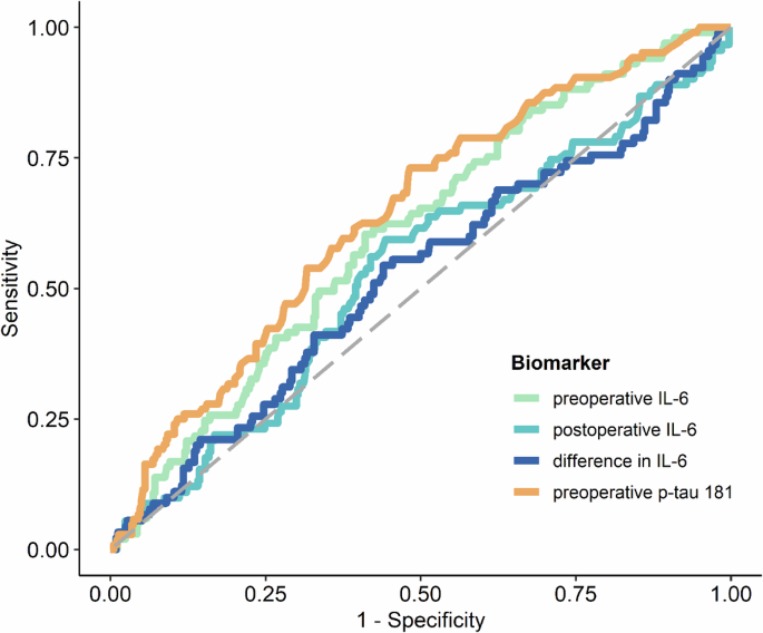
The levels of preoperative IL-6 and preoperative p-tau181 were identified as significant predictors of POD. This is illustrated in Fig. 1; Supplementary Table 4. Supplementary Figure 1 also show the log-transformed biomarker levels of IL-6 and p-tau181. ROC analysis yielded an AUC of 0.605 (95%-CI: 0.544, 0.663, p = 0.0018) for preoperative IL-6 levels and an AUC of 0.641 (95%-CI: 0.581, 0.698, p < 0.0001) for preoperative p-tau181. The optimal cut-off value for preoperative IL-6 was 4.71, demonstrating a sensitivity of 60.4% and a specificity of 58.9%, as detailed in supplementary Table 5A (for postoperative IL-6 cut off value, see Table 4B). The optimal cut-off value determined for preoperative p-tau 181 was 1.57, with a sensitivity of 61.5% and a specificity 60.7%, as reported in supplementary Table 5C. However, it was observed that POD could not be predicted based on postoperative IL-6 levels or the difference between postoperative and preoperative IL-6 levels, as indicated in supplementary Table 4, supplementary Figures 1B, C and Fig. 1. Furthermore, a linear mixed-effects model for IL-6 demonstrated that while time (p < 0.0001) and POD (p = 0.03) were significant factors, the interaction between time and POD was not significant (p = 0.09), as depicted in supplementary Figure 2. The mean group values in the difference of the log-transformed IL-6 levels for no POD were 1.809 (95%-CI: 1.71, 1.91, p < 0.0001) and 1.624 for POD (95%-CI: 1.43, 1.82, p < 0.0001).
ROC curves of preoperative IL-6 (orange), preoperative p-tau 181 (green), postoperative IL-6 (light blue) and the difference between post- and preoperative IL-6 (dark blue) blood levels for predicting POD following the CAM and CAM-ICU POD definition. Abbreviations: CAM = confusion assessment method, CAM-ICU = Confusion Assessment Method for the Intensive Care Unit, POD = postoperative delirium, IL-6 = interleukin 6, p-tau181 = phosphorylated tau protein 181.
Predicting postoperative delirium by combining plasma biomarkers and heart and brain as well as immunotherapy related factors
To identify possible associations among biomarkers and various heart and brain as well as immune system related factors, we conducted a multiple logistic regression analysis in three different models (Table 2A). In the first model, IL-6, age, sex, tumor, corticosteroids, colchicine and cytostatic drugs were included as explanatory variables in the analysis; we found that age and log-transformed preoperative IL-6 facilitated the prediction of POD (Table 2B and Fig. 2, Model 1). We investigated the immunotherapy-associated variables in a model with IL-6, since the activity of the inflammatory marker IL-6 can be influenced by immunotherapy. Our first model was able to predict POD with reasonable accuracy, achieving an AUC of 0.658 (95%-CI: 0.596, 0.714, p < 0.0001), as shown in Table 2B and Fig. 2, Model 1. Log p-tau181, age, gender, cognitive performance measured by MoCA and education were included as explanatory variables in our second model. It also included cognitive performance together with preoperative p-tau181 levels, as neurodegenerative processes are often associated with reduced cognition. This model revealed that log-transformed preoperative p-tau181, female sex, and cognitive performance were relevant factors. POD could be predicted with this model with moderate accuracy, namely an AUC of 0.694 (95%-CI: 0.637, 0.747, p < 0.0001, Table 2C, Fig. 2, Model 2). When we combined all explanatory variables (log-transformed IL-6, log-transformed p-tau181, age, sex, tumor, corticosteroids, colchicine, cytostatic drugs, MoCA findings, education, preoperative log IL-6 and preoperative p-tau 181 and female sex) into one model (Model 3), female sex, education > 10 years and cognitive performance (MoCA) proved to be relevant factors. However, the interaction between the blood biomarkers p-tau181 and IL-6 in blood plasma was not a relevant POD predictor (OR 0.87, 95%-CI: 0.48, 1.56, p = 0.63, Table 2, Model 3). With this combined model 3, POD was predictable with moderate accuracy with an AUC of 0.709 (95% CI: 0.651, 0.763, p < 0.0001; Table 2D, Fig. 2, Model 3).

Model 1: Plasma log transformed preoperative IL-6 in conjunction with age predict POD with an AUC of 0.658 (95%-CI, 0.596, 0.714, p < 0.0001). Model 2: log transformed preoperative IL-6 in conjunction with female sex and cognitive performance (MoCa assessment findings) predict POD with an AUC of 0.694 (95%-CI, 0.637, 0.747, p < 0.0001). Model 3: preoperative log-transformed levels of p-tau181 and IL-6, sex and cognitive performance determine POD prediction with an AUC of 0.710 (95%-CI, 0.651, 0.763, p < 0.0001). Abbreviation: AUC = area under the curve, CI = confidence interval, MoCa= Montreal Cognitive Assessment, ROC = receiver operating characteristics.
Predicting postoperative delirium taking a machine learning approach
Decision tree
To identify the most important guidelines for predicting POD, we created a decision showing four important rules. The rules were applied in the following sequence: (1) preoperative p-tau181 level greater than 1.4, (2) the presence of moderate or severe mitral valve disease, (3) a preoperative p-tau181 exceeding 1.8, and (4) preoperative IL-6 level above 5.8, as depicted in Fig. 3. The performance of this decision tree model was quantitatively evaluated, showing an AUC of 0.672 (95%-CI: 0.604, 0.735, p < 0.0001) on the training set and 0.642 (95%-CI: 0.537, 0.738, p = 0.0108) on the validation set. These results, along with detailed visual representations, are provided in supplementary Table 6, Fig. 3.

Decision tree with the four most predictive variables for POD, ie, preoperative p-tau181 value, preoperative IL-6 and severity of mitral valve disease. Abbreviation: POD = postoperative delirium, p-tau 181 = phosphorylated tau protein 181, IL-6 = interleukin 6.
LASSO
During the application of the LASSO machine learning procedure, non-zero regression coefficient estimates were observed for two variables: age and preoperative p-tau181 levels. The performance of the LASSO model in predicting POD was assessed using ROC analysis, which demonstrated an AUC of 0.751 (95%-CI: 0.686, 0.805, p < 0.0001) for the training and an AUC of 0.652 (95%-CI: 0.539, 0.747, p = 0.0086) for the validation set, reflecting a moderate level of prediction accuracy. These findings, along with the corresponding graphical representation, are detailed in supplementary Table 6 and Fig. 4A, B.

ROC analysis revealed that the classification model decision tree yielded significantly predictive accuracy of POD for the training (A) and validation (B) datasets [A, B: p < 0.05; AUC for the training dataset of 0.672 (95%-CI: 0.604, 0.735, p < 0.0001); AUC for the validation dataset of 0.642 (95%-CI: 0.537, 0.738, p = 0. 0108)]. LASSO also predicted POD accurately with an AUC of 0.751 (95%-CI: 0.686, 0.805, p < 0.0001) for the training dataset (A) and 0.652 (95%-CI: 0.538, 0.747, p = 0.0086) for the validation dataset (B). Abbreviations: CI = confidence interval, ROC = receiver operating characteristics, POD = postoperative delirium.