‘We’re glad to welcome and support Propair, a regional airline that, with its long operational history, understands those needs and values the opportunity to provide air service to the North Bay region’
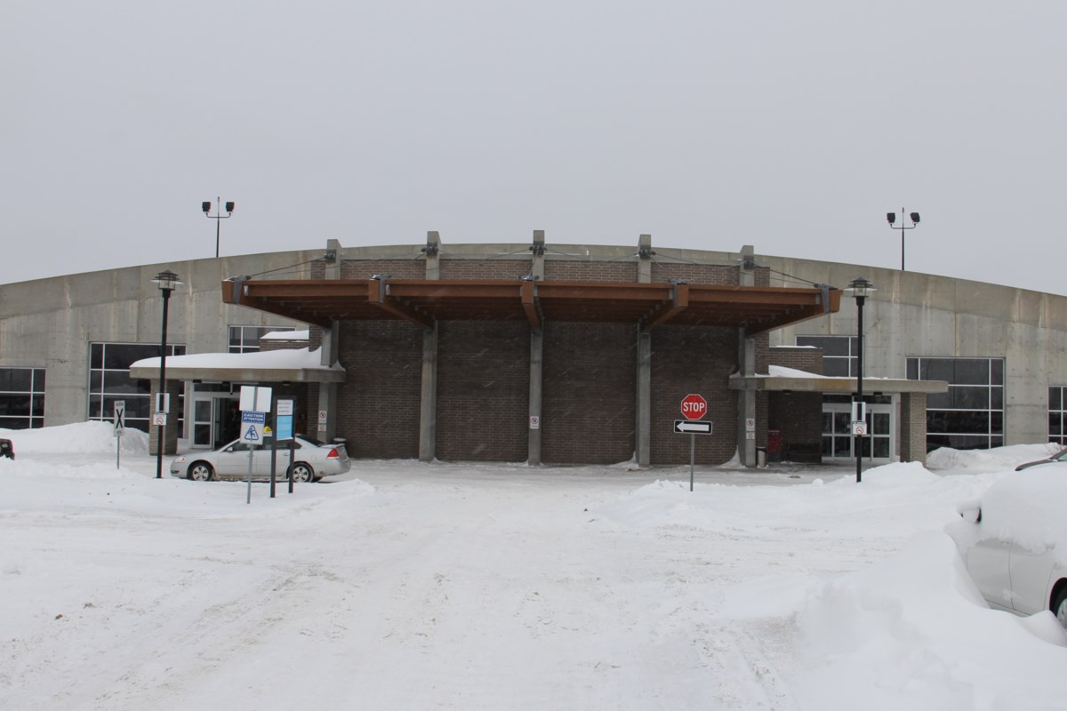
Bryan Avery says the Propair Airline, which will start offering flights from Jack Garland Airport in North Bay to Toronto, is welcome addition, and some good business news for the airport in 2026.
“It’s an exciting opportunity for the region, with service to Billy Bishop Toronto City Airport again, as well as an all-new connection with Rouyn-Noranda Airport,” said Avery, the Airport Manager at North Bay’s airport.
The new service is operated by Propair, a regional air carrier based in Northern Quebec with over 70 years of aviation experience.
These flights, offered five days a week, will begin in February 2026, and reservations are now available online at www.propair.ca.
See related: New airline coming to Jack Garland Airport
The new airline fills a void left by Air Canada, which announced in September 2025 that it would be leaving North Bay at the end of January 2026.
The Beechcraft 1900D aircraft, which accommodates up to 18 passengers, will operate regular flights from North Bay to Billy Bishop Toronto City Airport to better meet the needs of a wide range of travellers and facilitate connections to international flights.
Propair will also offer a shuttle service between Billy Bishop Airport and Toronto Pearson International Airport.
“We’re glad to welcome and support Propair, a regional airline that, with its long operational history, understands those needs and values the opportunity to provide air service to the North Bay region,” added Avery.
“With the information and comments we received during our traveller analysis in summer 2025, as well as in recent months, we knew that options to travel with greater flexibility were what was needed.”
Avery notes that Propair is not new to North Bay.
“In the past, they’ve operated charters to many airports such as ours to connect businesses,” said Avery.
“After a lot of work by all stakeholders, Propair is now introducing this regularly scheduled air service that everyone can book for business or liesure – today.
“Every ticket purchased with the airlines operating from North Bay Jack Garland Airport contributes to maintaining convenient air access for our region—an investment in our community’s future.”
The audio version of this article is generated by AI-based technology. Mispronunciations can occur. We are working with our partners to continually review and improve the results.
For years, oil tanker traffic has been prohibited off the waters of northern British Columbia in order to protect environmentally sensitive coastlines from disaster.
But the federal government is now open to the idea of changing its moratorium.
The debate over the future of the tanker ban arose from Prime Minister Mark Carney and Alberta Premier Danielle Smith signing a memorandum of understanding (MOU) in November that lays out the steps for a potential pipeline to carry oil from the Alberta to the Pacific coast.
Here’s what you need to know about the oil tanker moratorium and the area it’s meant to protect.
What is the ban on oil tanker traffic?
The federal government first imposed an oil tanker moratorium back in 1972 but it wasn’t legislated, as the Oil Tanker Moratorium Act, until 2019.
The ban covers an area that stretches from the northern tip off Vancouver Island to the B.C.-Alaska border.
The act prohibits oil tankers from stopping, loading or unloading in any port in the designated area.
It applies to vessels carrying a cargo of more than 12,500 metric tons of crude oil or persistent oil products, such as bitumen and Bunker C fuel, which dissipate slowly and can linger in the environment.
The moratorium does not apply to refined oil products, like gasoline, diesel and jet fuel, as well as liquefied natural gas (LNG).
Penalties for violating the Tanker Moratorium Act can include fines up to $5 million for each instance of non-compliance.
What’s the voluntary tanker exclusion zone?
The federal government established the voluntary tanker exclusion zone in the late 1980s. It offers a larger buffer zone between tankers and much of B.C.’s coast.
That boundary extends further off shore, about 100 km west of Haida Gwaii and roughly 40 km off Vancouver Island.
It’s aimed at U.S. tankers transporting oil between the Trans-Alaska Pipeline System marine terminal in Valdez, Alaska and refineries in Washington state.
“The size of the area was based on calculating the worst possible drift of a disabled tanker with a cargo, versus the time required for help to arrive,” Transport Canada explains on its website.
WATCH | Carney could change tanker moratorium:
Federal government agrees to possible B.C. tanker ban exemptions: sources
CBC News has confirmed that the federal government has agreed to possible exemptions to the tanker ban on B.C.’s northern coast as it discusses a new energy accord with Alberta.
How dangerous are the waters in moratorium area?
The Hecate Strait, famed for being treacherous, is often the focus of concerns about oil tanker traffic.
It separates Haida Gwaii from mainland B.C. and all types of boats, including fishing vessels, ferries and container ships, have run into problems in this stretch of water.
There is a “cocktail of risks” when it comes to navigating vessels in any area of open water, says Mariah McCooey, director of hydrography for the Pacific region of the Canadian Hydrographic Service (CHS) — a division of the science branch of the Department of Fisheries and Oceans that is tasked with supporting safe navigation.
But she explains that what makes the Hecate strait unique is that it’s particularly shallow, which contributes to big Pacific waves stacking up even higher.
WUDONG, a liquefied natural gas (LNG) tanker, fills up at an LNG Canada facility in Kitimat, B.C., on Nov. 13. The oil tanker moratorium does not prohibit vessels carrying LNG or refined oil products. (Ethan Cairns/The Canadian Press)
How do ships navigate the area?
Mariners are what McCooey calls “risk-assessing machines,” who use all available data to steer ships.
Navigation charts for areas off Haida Gwaii and the north coast of B.C. have greatly improved in the past 10 years thanks to new technology and data collection, she said.
Prior to that, McCooey explains, charts relied on survey data that dated back to 1912 and measured manually.
She says CHS now has 50 updated charts, covering hundreds of kilometres of coastline, using high quality sensors capable of collecting thousands of data points at one time and giving a clearer picture of what lies beneath the surface of the waters off northern B.C.
Any vessel travelling in the Hecate Strait would also rely on the knowledge of a specialized pilot who is mandated to be on board and guide ships from ports out to sea.
WATCH | Possible changes to oil tanker moratorium strikes fears on B.C.’s coast:
First Nations, experts warn of catastrophic risk in lifting B.C. oil tanker ban
A potential new oil pipeline from Alberta to B.C. is shedding light on the dangerous B.C. waters that tankers would have to navigate if it’s built. CBC’s Janella Hamilton dives into the implications and the worries.
Who’s for and against the moratorium?
Those who want the tanker ban lifted or changed — including Alberta’s oil sector, Premier Smith and federal Conservative leader Pierre Poilievre — argue it hinders Alberta’s ability to export its oil to key markets in Asia.
Supporters of the moratorium, including First Nations and environmental groups, say the ban is vital to protecting environmentally sensitive coastal areas and critical marine ecosystem that are key to both the provincial economy and Indigenous ways of life.
“There is no technology that can clean up an oil spill at sea or in a salmon river,” Coastal First Nations said in a statement emailed to CBC News last month, calling the moratorium a “matter of national responsibility.”
B.C.’s NDP-led government also supports the moratorium, and in November, Premier David Eby signed a declaration, along with Coastal First Nations, urging Ottawa to keep the oil tanker ban in place.
WATCH | Political and environmental pushback to a potential pipeline partnership:
The Breakdown | Carney’s Alberta pipeline partnership
The National’s At Issue panel breaks down Prime Minister Mark Carney and Alberta Premier Danielle Smith’s partnership to build a new pipeline out of Alberta and the political and environmental pushback it sparked.
TikTok has signed a deal to sell its U.S. operations to a group of investors led by Larry Ellison, the billionaire ally of Trump whose family media and entertainment empire just got bigger.
AYESHA RASCOE, HOST:
TikTok’s CEO says a deal has been signed to sell TikTok’s U.S. business to a group of mostly American investors. One of the lead billionaires behind the new entity is Larry Ellison, the chief executive of tech company Oracle. Ellison is a longtime ally of President Trump. NPR’s Bobby Allyn joins us to discuss what this new ownership means for the Ellison family’s growing business empire and the future of social media. Hi, Bobby.
BOBBY ALLYN, BYLINE: Hey, Ayesha.
RASCOE: So the American version of TikTok is about to get new owners. Tell us more about this deal.
ALLYN: Sure. I obtained an internal memo sent by TikTok’s CEO, Shou Chew, and he lays out exactly what’s going on here. And he says a new U.S. company will be established to monitor TikTok’s data flows and how the algorithm is working. So, you know, what’s being amplified and what’s not. And the group overseeing all of this will be a private equity firm called Silver Lake, the United Arab Emirates-backed fund MGX and Oracle, the software and data center company run by Larry Ellison. Now, TikTok’s parent company, ByteDance, in Beijing will still have a minority stake, and existing TikTok investors are also going to get some equity in this deal. But Larry Ellison, you know, is going to be a really pivotal figure in all of this.
RASCOE: So how did Ellison become a key player in the future of TikTok?
ALLYN: Yeah. You know, when lawmakers in Washington really started putting the heat on TikTok over its ties to China years ago, Ellison saw an opportunity. He really stepped up, and he offered to migrate all of Americans’ TikTok data over to Oracle servers. Oracle moved its headquarters to Austin, and TikTok started calling its plan to cordon off China from American TikTok users Project Texas as a nod to just how important Oracle would be. So that’s on the technical side. But on the political side, he’s, for years, been a huge supporter of President Trump. And in his second term, Ellison has become one of the most visible leaders in Trump’s orbit. And, you know, Ayesha, it’s worth mentioning here that this is a late career move for Ellison. He’s 81 years old, but TikTok is now in the stable of the Ellison family’s media and entertainment empire.
RASCOE: What do the Ellisons now have control over?
ALLYN: Yeah. Larry Ellison’s son, David, is the CEO and chairman of Paramount Skydance, which controls CBS News, Paramount Pictures, Paramount+ and more. And now the Ellisons are making a hostile bid to try to acquire Warner Brothers Discovery. And to get a hint of where they lean politically, I mean, look no further than to Paramount’s acquisition this year of The Free Press, which is a right-wing online website run by Bari Weiss that has positioned itself as the leading anti-woke voice on the internet.
RASCOE: Well, I mean, back to TikTok, could there be any changes in store for American users with the app now under the Ellison family’s control?
ALLYN: Yeah, and that’s the big question here. The internal memo that I got about the deal, you know, says that this new Ellison-led entity means that Ellison and these other investors are going to control content moderation on TikTok. So what’s allowed, what’s not, what you and I can post. And free-speech experts I talked to said that is no small thing. I mean, I started covering TikTok, Ayesha, like, six years ago, when its troubles began. And back then, everyone was super worried about this notion that China could censor what is allowed on the app. But now TikTok watchers are wondering if the Ellisons’ new content rules will make some other people feel like – that their voices are being censored. So that’s definitely something we’ll be watching going into the future.
RASCOE: That’s NPR’s Bobby Allyn. Thank you so much.
Accuracy and availability of NPR transcripts may vary. Transcript text may be revised to correct errors or match updates to audio. Audio on npr.org may be edited after its original broadcast or publication. The authoritative record of NPR’s programming is the audio record.
Miss something this week? Don’t panic. CBC’s Marketplace rounds up the consumer and health news you need.
Want this in your inbox? Get the Marketplacenewsletter every Friday.
Happy holidays! We’ll be back in 2026
As the holidays near, our newsletter will be taking a short hiatus — but we’ll still be on the lookout for consumer news, tips and insider info to help you save cash and stay healthy.
We’ll be back in 2026 with more of this newsletter on Jan. 9 and new episodes of Marketplace starting Jan. 16.
Air Canada wins court battle to quash $2,000 payout to passenger for delayed luggage
A dispute between Air Canada and a passenger has been sent back to the Canadian Transportation Agency, the country’s transport regulator, for a new officer to reassess the compensation claim. (Mike Hillman/CBC)
Air Canada has successfully overturned a Canadian Transportation Agency (CTA) decision requiring the airline to pay a passenger $2,079 for delayed baggage.
After an 11-month court battle launched by Air Canada, Federal Court Justice Michael Manson ruled that a CTA officer’s 2024 decision was unreasonable. The matter has been sent back to the CTA, Canada’s transport regulator, for a new officer to reassess the compensation claim.
The case originates from a 2022 flight Alaa Tannous and his wife, Nancy, took from their home city of Toronto to Vancouver. Their checked baggage arrived one day after they did.
Air Canada originally offered Tannous $250 compensation. Dissatisfied with the amount, he filed a complaint with the CTA.
According to court documents, Air Canada argued the CTA’s order to award Tannous $2,079 was flawed, because the purchases he made to replace the items in his missing suitcase “were excessive, included luxury items,” and some goods were bought after the suitcase was returned.
In his decision, Manson agreed that the CTA ruling was questionable, because it included a portion of the later purchases.
“The officer’s reasons do not address nor show any common sense on why post-delivery purchases were causally linked to the delay,” he wrote.
Air Canada told CBC News in an email that it’s satisfied with the judge’s decision.
Tannous said Air Canada served him with court papers on Christmas Eve in 2024. He said he did not hire a lawyer or participate in the court case, because he felt it was a waste of money and time. He declined to comment on the outcome of the case except to point out that it’s still active.
Read more from CBC’s Sophia Harris.
Canada’s inflation rate stayed flat in November but grocery prices grew at fastest pace in nearly 2 years
WATCH | Why beef prices could continue to climb in 2026:
Why beef prices keep going up
High beef prices are expected to continue to climb in 2026. For The National, CBC’s Paula Duhatschek breaks down what’s making meat so expensive and what it will take to stabilize the Canadian market.
Canada’s annual inflation rate was unchanged in November, but grocery inflation reached its highest rate in nearly two years, Statistics Canada said on Monday.
While the overall inflation rate came in at 2.2 per cent, in November, food costs increased by 4.7 per cent compared to this time last year.
That marked the largest increase to grocery price growth since December 2023.
Fresh fruit — especially pricier berries — drove the increase, as did “other food preparations” (a category that mostly includes processed foods).
Coffee prices remain stubbornly high, having increased 27.8 per cent on a yearly basis in November. The trend has been ongoing as coffee-growing countries face adverse weather conditions and U.S. tariffs.
Meanwhile, fresh and frozen beef — up 17.7 per cent last month — continued to weigh on inflation, with prices driven up partly because cattle inventories are shrinking across North America.
Marketplace will tackle this topic in January with an investigation about how grocery stores themselves are driving the increase in the cost of food.
Read more from CBC’s Jenna Benchetrit.
AI is skyrocketing the price of RAM. Computers, phones and tablets could be next
RAM memory chips are becoming more expensive. (CBC News)
From computers to cellphones and even certain features in cars, a lot of electronics rely on random-access memory, or RAM. It’s the fundamental hardware your computer processor needs to run applications, open files and let you surf the internet.
But if you’ve been in the market recently for RAM, you’ve probably noticed a major spike in prices as memory manufacturers pivot more of their production capacity away from consumer products to supplying AI companies instead, which are rapidly building data centres that need massive amounts of memory to operate.
“Prices have absolutely skyrocketed since the beginning of November,” Mark Chen, store manager at Uniway Computers, which sells custom-built PCs with RAM in Calgary, told CBC News in an email.
Back in October, Chen said he could find a 32GB DDR5 memory kit for under $130. By mid-November, the price had more than doubled to around $300.
Now, Chen says, it’s difficult to find that same memory kit for less than $400.
“Everything that uses memory, the prices are going to go up,” Willy Shih, a professor of management practice at Harvard Business School, said.
That’s essentially every electronic product from cellphones to smart fridges to modern cars.
Read more from CBC’s Rukhsar Ali.
What else is going on?
Lawyer who admitted stealing millions of dollars from homeowners is disbarred
Singa Bui forged bank statements to hide theft from auditors, tribunal hears
Via Rail CEO stepping down as Crown corporation faces increasing scrutiny
Retirement comes amid criticism of rising ticket prices and delays
Air Transat’s parent company reports $12.5M loss in latest quarter
Airline owner’s revenue increased by 1.5% compared with a year ago
National home sales fell in November with housing activity in ‘holding pattern,’ says CREA
Some sellers making price concessions to get end-of-year deals done, says economist
Thinking about going off an antidepressant? Here’s what experts want you to know about doing so safely
Many Canadians use antidepressants, but it’s not always clear when to stop
Marketplace needs your help!
Have you complained to the consumer protection office in your province or territory? If so, we want to know how it went. Email us at marketplace@cbc.ca.
Are you planning on cancelling your cell, cable or internet service? Before you do, Marketplace wants to hear from you! Email us at marketplace@cbc.ca.
Catch up on past episodes of Marketplace onCBC Gem.
In this podcast, the discussion will explore what GP staking really means for fund managers and investors, examine key financing structures such as fund finance, rated feeders, and CFOs, and delve into value creation strategies. It will also highlight the motivations, opportunities, and strategic solutions offered by Investcorp, providing listeners with a comprehensive understanding of these critical aspects of private market investing.
This First Person article is the experience of Itrat Anwar, a newcomer from Bangladesh who now calls Steinbach, Man., his home. For more information about CBC’s First Person stories, please see this FAQ. You can read more First Person articles here.
This Christmas, we hold each other close, thankful for the life we’ve built here in Canada. It’s a season of warmth, joy and togetherness, a time for family.
But for us, Christmas brings a deep sense of longing. This will be the fourth year we’ve spent it far from our parents, separated by thousands of kilometres.
We long for them to feel the warmth of their grandchildren’s embrace, not just through a screen, but in person. There’s still an empty seat at our table.
We’re surrounded by friends who feel like family and we remind ourselves often: We are lucky.
But even gratitude can’t silence some kinds of longing.
We laughed, we cried, we waved at the screen and pretended we were there.– Itrat Anwar
My wife, Halyna, lost her mother the same month the Russian invasion of Ukraine began, while she was pregnant. The grief, the fear, the constant air raid alarms — it was more than any heart should have to bear.
After days filled with uncertainty and danger, she finally escaped the war with a harrowing train journey, desperately seeking safety.
Halyna says those days were the most terrifying of her life, and she still has nightmares. She believes only those who’ve lived through it can truly understand the depth of that fear.
It was during this difficult time that Halyna met my parents for the first time in Bangladesh. Despite the heavy sorrow she was carrying, a bond quickly formed between them.
My mother welcomed her not just as a daughter-in-law, but as a daughter who had come home. The love and warmth they showed her helped soften the grief she had been holding onto.
For the first time since losing her own mother, Halyna began to feel a sense of family again, a feeling she had thought lost forever.
After Halyna Kukurudz, left, met her mother-in-law, Israt Jahan, right, she ‘began to feel a sense of family again,’ Itrat Anwar says. (Submitted by Itrat Anwar)
When we moved to Canada, we carried with us a simple dream: that one day, we would bring our parents here too, and be together again as a family — but life had different plans.
Just as we were searching for ways to make that dream a reality, we were blindsided by news that would change everything: my mother was diagnosed with cancer.
For months, she endured chemotherapy, surgery and radiation. Now, she’s undergoing additional treatments and continues to fight.
Her strength has always been an inspiration to us, but watching her go through this from across the ocean has left us feeling helpless. Sometimes, we believe the only reason she’s fighting so hard, staying strong, is because she wants to see her grandchildren.
The distance has never felt heavier.
Meanwhile, our children are growing quickly. Neither of them has met their grandparents in person, not once. Their relationship with them exists only through glowing screens and grainy video calls.
Sometimes, they hug the screen and call them “My nanu,” (grandma), kissing it as if trying to bridge the kilometres between them. It’s a bittersweet moment — sweet in its innocence, yet heartbreaking in the realization of how far apart we are.
Recently, my only brother got married. Even though we were so far away and it was midnight here, we watched the ceremony over a video call. We laughed, we cried, we waved at the screen and pretended we were there.
Life here in Canada is good, truly good. I work to support the family, while my wife cares for our little ones at home, eagerly waiting for the day when our parents can finally be here with us. She’s also ready to return to work, so we can better manage financially.
Some days, though, are hard. The weight of rent, bills and car payments can feel overwhelming. Flying across the world to visit our parents isn’t something we can manage right now, and bringing them here still feels like a distant dream.
We worry about their safety in Bangladesh. The year 2024 was chaotic, and the political situation is growing more unstable. The upcoming national elections could bring even more violence.
The images from this time are unsettling, and if you saw them, they would scare you. I’ve grown up amid political unrest, and it has always been volatile. I was lucky to survive several close calls myself.
We dream. We hope. And we hold our parents close, across continents.– Itrat Anwar
This fear, this uncertainty, is something we carry with us every day. And though we are safe here in Canada, the ache of being far from our loved ones only grows stronger. We know we’re not alone in this. So many immigrant families carry the same quiet pain.
Still, we imagine the day when our children will finally run into their grandparents’ arms, not through a screen, but in a real embrace — one filled with warmth, tears and all the years we’ve been waiting for this.
Next year, we’ll celebrate together. Maybe next year, those empty spaces at our table will finally be filled. And until then, we dream. We hope. And we hold our parents close, across continents, across screens, across every mile between us.
Simply sign up to the Equities myFT Digest — delivered directly to your inbox.
The traditional market “Santa rally” — a seasonal phenomenon in which stocks often rally through November and December — has been conspicuous by its absence this year, as fears about massive spending on infrastructure by highly valued artificial intelligence companies have weighed on investors’ minds.
“December is often synonymous with buoyant equities,” wrote analysts at Bank of America. “But this year’s backdrop is anything but ordinary. From AI-driven volatility to shifting Fed expectations . . . investors are navigating a landscape where traditional year-end patterns could be challenged.”
On average, since 1928, the S&P 500 has risen 4 per cent between October 28 and New Year’s Eve, Deutsche Bank analysis showed. This year, both the S&P 500 and the tech-heavy Nasdaq Composite are in negative territory in that period so far.
Earnings from Oracle and Broadcom, both of which fell short of analysts’ lofty expectations, were the catalysts for the most recent market wobbles. Oracle’s share price has fallen about 45 per cent from its September peak and, in a sign of contagion, Nvidia is down about 15 per cent since the start of November.
But despite the recent jitters, global equity markets have still logged double-digit gains this year.
Mislav Matejka, head of global and European equity strategy at JPMorgan, suggested that investors might “square positions and reduce directional risk into the end of the year” to lock in their 2025 gains. “You don’t have a tailwind in the very near term,” he suggested.
While a full reversal of recent losses may be off the cards, the final trading sessions of the year are unlikely to do damage to a very strong year for markets. Emily Herbert
How much did US growth slow in the third quarter?
Investors will get a final pre-Christmas reading on the health of the world’s largest economy this week, and Tuesday’s GDP data is expected to paint a buoyant picture despite growth slowing.
Economists polled by Reuters forecast that output expanded at an annualised rate of 3.2 per cent in the third quarter, easing from 3.8 per cent in the previous three months but comfortably ahead of the 2.3 per cent pace recorded a year earlier. If realised, the data would reinforce the view that the US economy continues to outperform its peers even as growth moderates.
The release has been delayed by the federal government shutdown earlier this year, which also caused the Bureau of Economic Analysis to scrap its customary advance estimate for the third quarter. Instead, it will publish a combined first and second estimate, heightening recent uncertainty about official data.
Much of the third quarter’s momentum is expected to have come from capital spending linked to the artificial intelligence boom, particularly investment in data centres and computing equipment. Matthew Martin, senior US economist at Oxford Economics, estimates that such investment has added roughly $60bn to real GDP over the past two years and said this week that “this is only likely to grow”. Investors will be keen to assess how concentrated that strength has been, and whether it reflects a broader uplift in business investment.
Household consumption will be another focal point. Consumer spending has remained resilient despite elevated interest rates and early signs of cooling in the labour market, providing a crucial buffer against slowing growth elsewhere. Investors will look closely at whether services spending continued to offset weakness in goods demand as households adjusted to tighter financial conditions.
Yet confidence in the data itself may be fragile. Restrictions placed on the Bureau of Labor Statistics during the government shutdown have already raised doubts about recent economic releases. Markets barely reacted to data this week showing a sharp slowdown in consumer price inflation, with investors discounting figures compiled amid gaps in survey collection — a scepticism that may also colour the reception of next week’s GDP report. Kate Duguid
Is Australia moving closer to a rate rise?
When the Reserve Bank of Australia decided earlier this month to leave its policy interest rate unchanged at 3.6 per cent, it also signalled a “more broadly based pick-up in inflation”, intensifying speculation that its next move would be to raise rates, after three cuts this year.
Traders are ascribing a roughly 25 per cent chance to the RBA’s first rise coming in February, according to levels implied by derivatives markets. The minutes of the December meeting, to be released on Tuesday, will be pored over by investors for anything that supports or contradicts that view.
Australia has been one example, along with Canada and others, where global rates traders have moved to call the end of the rate-cutting cycle, prompted by stubborn inflation and stronger than expected economic data.
RBA governor Michele Bullock said on the day of the December decision that the rate-setting board would “do what it thinks it needs to do” to get inflation back to the 2.5 per cent midpoint of its target range. Inflation was running at 3.8 per cent in October.
“We expect the minutes to contain information on what the board would need to see to produce a rate hike,” said analysts at Citi. The minutes will also be closely watched by rate-setters elsewhere, for whom Australia might be a sign of things to come. Ian Smith