Category: 3. Business

17 December 2025

• Aggregate Common Equity Tier 1 ratio at 16.10% in third quarter of 2025, compared with 16.12% in previous quarter and 15.73% one year ago
• Aggregated annualised return on equity at 9.88% in third quarter of 2025, down from 10.11% in previous quarter and 10.09% one year ago
• Aggregate non-performing loans ratio (excluding cash balances) at 2.22% in third quarter of 2025, unchanged from previous quarter and down from to 2.31% one year ago
• Liquidity coverage ratio at 156.73% in third quarter of 2025, down from 157.88% in previous quarter and 158.50% one year ago

Capital adequacy

Capital ratios interactive report

In the third quarter of 2025, the aggregate Common Equity Tier 1 (CET1) ratio and the Tier 1 ratio of significant institutions (banks supervised directly by the ECB) were slightly lower than in the previous quarter. The aggregate CET1 ratio stood at 16.10% and the aggregate Tier 1 ratio stood at 17.59%. At the same time, the aggregate total capital ratio remained stable at 20.24% compared to the previous quarter. Across countries, the CET1 ratio ranged from 13.28% in Spain to 23.12% in Lithuania in the third quarter of 2025.

Asset quality

Non-performing loans interactive report

The non-performing loans (NPL) ratio excluding cash balances at central banks and other demand deposits stood at 2.22% in the third quarter of 2025. The stock of NPLs (numerator) increased by €1.49 billion (0.42%), and at the same time the total amount of loans and advances (denominator) rose by €30.95 billion (0.19%). As a result, the ratio remained stable compared to the previous quarter.

At sector level, the NPL ratio for loans to households stood at 2.16%, unchanged from the previous quarter and down from 2.25% a year ago. At the same time, for loans to non-financial corporations (NFCs), the ratio stood at 3.51%, compared with 3.50% in the previous quarter and 3.65% one year ago. Considering the NFC portfolio by segment, the NPL ratio for loans collateralised by commercial immovable property stood at 4.58%, compared with 4.55% both in the previous quarter and one year ago. The NPL ratio stood at 4.88% for loans to small and medium-sized enterprises, compared with 4.85% in the previous quarter and 4.88% one year ago.

Aggregate stage 2 loans as a share of total loans decreased to 9.49% from 9.59% in the previous quarter. The ratio for loans to NFCs decreased to 13.55% and the ratio for loans to households decreased to 9.41% from 13.65% and 9.47% in the previous quarter, respectively.

Profitability

Profitability interactive report

The aggregate annualised return on equity stood at 9.88% in the third quarter of 2025 compared with 10.11% in the previous quarter and 10.09% one year ago. The return on equity across countries ranged from 6.82% in France to 16.66% in Lithuania in the third quarter of 2025. At the same time, the aggregate net interest margin was basically unchanged compared to the previous quarter.

Liquidity

Liquidity interactive report

The aggregate liquidity coverage ratio decreased to 156.73% in the third quarter of 2025, down from 157.88% in the previous quarter and 158.50% one year ago. This downward trend was driven mainly by an increase of €37 billion (+1.15%) in the net liquidity outflow compared to the previous quarter.

Factors affecting changes

Supervisory banking statistics are calculated by aggregating the data reported by banks which report COREP (capital adequacy information) and FINREP (financial information) data at the relevant point in time. Consequently, changes from one quarter to the next can be influenced by the following factors:

• changes in the sample of reporting institutions;
• mergers and acquisitions;
• reclassifications (e.g. portfolio shifts as a result of certain assets being reclassified from one accounting portfolio to another).

For media queries, please contact Benoit Deeg, tel.: +491721683704.

Notes

• The complete set of supervisory banking statistics with additional quantitative risk indicators is available on the ECB’s banking supervision website. The time series are also available for download from the ECB Data Portal.

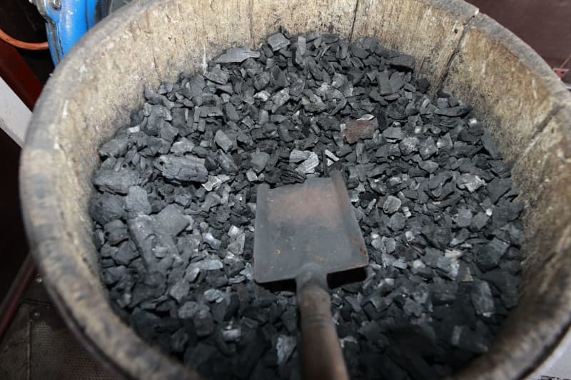
Global coal demand is expected to reach a new record high this year, the International Energy Agency (IEA) forecast on Wednesday, despite diverging regional trends in consumption.

In its annual coal market report, the IEA said global coal use is projected to rise by 0.5% to 8.85 billion tons this year.

In the United States, where demand has declined in recent years, consumption is set to increase by around 8% this year. The IEA attributed this to higher natural gas prices and a slowdown in the retirement of coal-fired power plants under the administration of President Donald Trump.

In the European Union, coal demand in 2025 fell by significantly less than in the previous two years, as lower output from wind and hydropower in the first half of the year led to greater reliance on coal-fired generation.

India, which typically contributes to growth in global demand, is expected to have generated less energy from coal this year. The IEA said an early and intense monsoon season reduced electricity demand while boosting hydropower output.

Looking ahead, the Paris-based IEA said its forecast shows global coal use plateauing in the coming years and then starting to tick lower by 2030.

Demand in China is expected to ease slightly by 2030 as renewable energy capacity expands rapidly. By contrast, the agency said India is likely to see the largest increase in coal consumption over the coming years.

The NEA held the Bridging Law and Technology: International Workshop for the Deployment of Small Modular Reactors (SMRs) from 8-10 December 2025 in Stockholm, Sweden. Co-organised with the Government of Sweden, the event brought together more than 200 legal, technical and policy experts to discuss the unique legal challenges posed by advancements in small modular, transportable, maritime, and generation IV reactors and identify potential paths forward.

The workshop was structured into five thematic sessions, combining keynote addresses, panel discussions and interactive Q&A segments. Focusing on authorising SMR designs, SMR pre-licensing and licensing challenges, factory manufacturing, mobile reactors and transportation, maritime applications, and fuel cycle, waste management and decommissioning, high-level speakers set the tone by emphasising the importance of bridging legal frameworks with technological innovation. Panels featured experts from governments, regulatory bodies, industry and academia, who discussed practical approaches to licensing SMRs, managing liability, and fostering international co-operation. Using a highly interactive format, every participant was encouraged to contribute their diverse expertise to directly shape the discussions and outcomes. The exchanges underscored the urgency of collaborative solutions and highlighted best practices from member countries.

 

In her opening remarks, Maja Lundbäck, State Secretary to Minister for Energy, Business and Industry Ebba Busch, Government of Sweden, highlighted the role of nuclear energy in ensuring energy security and supply in Sweden. “Access to energy at reasonable prices when and where it is needed is a democratic issue and necessary for building a sustainable society,” she noted. “Sweden is back when it comes to nuclear power.”

 

Maja Lundbäck, State Secretary to Minister for Energy, Business and Industry Ebba Busch, Government of Sweden

Daniel Westlén, State Secretary to Minister for Climate and the Environment Romina Pourmokhtari, shed light on the latest regulatory developments in Sweden, noting that “The government is reviewing all legislation related to nuclear power to enable the deployment of new reactors.”

Kimberly Sexton Nick, Head of the NEA Division of Nuclear Law, noted in her welcome remarks that “Legal and regulatory issues cannot be addressed in a vacuum, only by lawyers or only by technical experts or only by policymakers. The walls separating law, policy and technical expertise must be removed and only through sustained and committed communication and collaboration can those in the nuclear field chart a path forward.”

 

Daniel Westlén, State Secretary to Minister for Climate and the Environment Romina Pourmokhtari, and Kimberly Sexton Nick, Head of the NEA Division of Nuclear Law

Paul Bowden, the workshop moderator, set the tone stating that “The challenges associated with SMR deployment cannot be solved only with national solutions. The final goal of this workshop is to move beyond our own borders to see transnational opportunities and potential international approaches to problem solving.”

   

The workshop featured multiple panel discussions with experts from industry, government, academia and law fields

 

Fireside chat with Elena Santer, Secretary for the Espoo Convention and the SEA Protocol, UNECE, moderated by Paul Bowden

Preparatory work

In the months leading up to the workshop, extensive preparatory efforts were undertaken to ensure meaningful dialogue and actionable outcomes. Central to this process were the thematic working groups, which convened virtually in September, October, and November. These groups were led by co-chairs representing the NEA’s standing technical committees and they provided participants with early engagement opportunities, fostering collaboration across jurisdictions and disciplines. Their mandate included identifying key challenges, drafting targeted questions, and developing discussion papers summarising legal and technical frameworks relevant to SMR deployment.

Ultimately, the working groups produced comprehensive background papers that served as the foundation for workshop discussions. These documents synthesised survey results, national presentations, and group deliberations, highlighting critical issues such as the need to adapt existing frameworks (often built for large light water reactors) to advanced designs, while keeping predictability and safety outcomes front and centre. They also explored opportunities for international collaboration, including on issues related to manufacturing, transport and maritime regimes. These papers were instrumental in aligning participants on shared objectives and ensuring informed, constructive exchanges during the workshop.

Looking ahead: From dialogue to action

The insights generated during the workshop will inform future NEA initiatives aimed at supporting member countries in navigating legal and technical challenges associated with SMRs. While working group products remain restricted to participants until the official publication of the workshop proceedings in 2026, the collaborative spirit and knowledge exchange fostered through this process mark a significant step toward cross-border opportunities for innovative solutions. The NEA remains committed to facilitating these conversations and driving progress in nuclear law and technology.

Orange Money Group and Visa announce a strategic partnership aimed at accelerating online payments and democratizing access to financial services across Africa and the Middle East.

Already successfully deployed in Botswana, Madagascar, and Jordan, where the partnership is renewed, the virtual visa card has been recently launched by Orange Money Côte d’Ivoire. This launch was a success and perfectly illustrates our shared vision with Visa for a more inclusive and accessible financial ecosystem.  

This partnership marks a new milestone in the shared ambition of the two companies: to provide millions of users with a simple, secure, and internationally recognized payment solution.

Building on the success in these countries, it will be gradually rolled out to new markets such as Guinea, Burkina Faso, and the Democratic Republic of Congo.

Directly accessible from the Max it app, the Orange Money Visa virtual card allows users to instantly create a card that can be funded anytime from their Orange Money account, enabling secure online payments on local and international websites. A physical card will also be made available at authorized Orange Money points of sale at a later stage.

Orange Money is proud to partner with Visa, given its global expertise in secure digital payments and its extensive international acceptance network—ensuring Orange Money users enjoy a seamless and trusted payment experience wherever they are.

For Orange Money, this partnership is fully aligned with its mission to promote financial inclusion—simplifying access to digital services and empowering everyone to participate fully in the digital economy, regardless of their country or device.

Thierry Millet, CEO, Orange Money Group comments: “Thanks to Orange Money, our 45 million customers can make everyday payments at millions of physical retail locations and with online merchants in their country. Whether they are individuals or entrepreneurs, they can now create their virtual Visa card in just a few seconds and make international online payments across the Visa network. This is the first step in this strategic partnership, which will help make Orange Money a widely accepted payment method, from major online platforms to local neighborhood merchants.”

Ismahill Diaby, Vice-President, General Manager – Western and Central Francophone & Lusophone Africa, Visa comments: “We’re excited to partner with Orange Money to bring the advantages of the digital economy to millions of people across Africa. By combining Visa’s trusted technology with Orange Money’s local reach, this partnership offers a simple, secure way for more people and small businesses to pay online—helping them participate confidently in everyday commerce.”

With over 173 million customers and 45 million active accounts across 17 countries in Africa, Orange continues to drive digital and financial transformation across the continent, supported by Visa’s trusted technology.

 

About Orange Money Group
Orange Money, a pioneering solution for financial inclusion, is used every month by more than 45 million people across 17 countries in Africa and the Middle East. Orange Money Group, in coordination with local Orange Money entities and Orange Bank Africa, is responsible for defining the mobile financial services strategy for the Middle East and Africa region. It provides local entities with operational support to help them accelerate their growth, establish new partnerships, support their compliance plans, and develop new value-added activities that meet market expectations.

About Orange Middle-East and Africa (OMEA)
Orange is present in 17 countries in Africa and the Middle East and has 173 million customers at 30 november 2025. With 7.7 billion euros of revenues in 2024, Orange MEA is the first growth area in the Orange group. Orange Money, its flagship mobile-based money transfer and financial services offer is available in 17 countries and has more than 100 million customers. Orange, multi-services operator, key partner of the digital transformation provides its expertise to support the development of new digital services in Africa and the Middle East.

About Visa
Visa (NYSE: V) is a world leader in digital payments, facilitating transactions between consumers, merchants, financial institutions and government entities in more than 200 countries and territories. Our mission is to connect the world through the most innovative, convenient, reliable and secure payments network, enabling people, businesses and economies to thrive. We believe that economies that include everyone everywhere, lift everyone everywhere, and we see access as fundamental to the future of the movement of money. Find out more about Visa.com.

Islamabad: Pakistan is set to roll out a locally developed secure messaging app, “Beep,” for government employees in the coming months, local media reported on Wednesday.

The National Assembly Standing Committee on Information Technology and Telecom was informed on Tuesday that the messaging app inspired by the Chinese social media platform WeChat is almost ready for launch and is expected to meet the project deadline of June 30, 2026, the Dawn newspaper reported.

National Information Technology Board (NITB) Chief Executive Faisal Iqbal Ratyal said that “Beep” had been locally developed and certified by relevant government agencies for official use, such as the National Computer Emergency Response Team (NCERT), which has formally cleared the application for official use.

The Standing Committee Chairman, Syed Aminul Haque, directed the NITB to ensure the timely rollout of the application.

“The purpose of launching Beep is to provide a secure messaging platform for public sector employees nationwide,” Ratyal told the committee. He added the launch would take place in a phased manner, starting with federal ministries and associated departments.

The app will be rolled out in the next two months and will be integrated with Pakistan’s federal e-Office system, enabling secure messaging, document sharing and workflow coordination within government institutions.

According to the NITB, Beep will offer end-to-end encryption for text messages as well as video calls used by government officials.

Ratyal stressed that additional security features had been incorporated to address the concerns raised by the committee members amid recent global incidents that underscored vulnerabilities in digital platforms regarding data security and the protection of official communications.

Beep’s encryption standards had been strengthened to make it suitable for sensitive discussions, Ratyal added.

The platform would operate on a usage-based fee model, and efforts were underway to make it financially self-sustaining over time, said the NITB chief.

Officials said Beep’s servers would be based in Pakistan, with stricter security safeguards inspired by WeChat, while noting that although WhatsApp is a widely used platform for voice calls, video calls and media sharing, its data servers are located outside the country.

The committee was also briefed that the federal e-Office system had been introduced to reduce paperwork and improve transparency, and that integrating Beep was expected to strengthen internal coordination and reduce operational risks.

(Except for the headline, this article has not been edited by FPJ’s editorial team and is auto-generated from an agency feed.)