Eisai Presents New Data on the Continued and Expanding Benefit of LEQEMBI® (lecanemab-irmb) Maintenance Treatment in Early Alzheimer’s Disease at the Clinical Trials on Alzheimer’s Disease (CTAD) Conference 2025 Biogen
CTAD 2025: Lecanemab Boosts CSF Aβ Protofibrils, Confirming Target Engagement and Pharmacodynamic Effect Patient Care Online
New data confirm pharmacological effect of Leqembi, says Eisai The Pharma Letter
Biogen and Eisai Present New LEQEMBI Biomarker Data at Clinical Trials on Alzheimer’s Disease 2025 Conference MarketScreener
Lecanemab shows effect on Alzheimer’s biomarkers in new study Investing.com
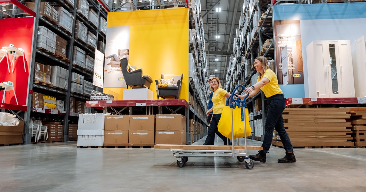
The long-anticipated store and its 500 co-workers welcomed crowds of excited Kiwis. Once through the doors, customers experienced styled room-sets and more than 7,500 products, convenient services, and plenty of inspiration.
For the first time when opening a new market, IKEA has set up 29 pick-up points across the country, where customers can collect their purchases even more affordably. The new IKEA store in Auckland, pick-up points, online and remote sales complement each other in an omnichannel way, allowing the Swedish retailer to get closer to the shopping preferences of New Zealanders. In addition, a Buy Back service is available at the store from day one – even for non-IKEA products – supporting circular living and reducing waste.
“I’m proud we are now open both in-store and online. We appreciate the excitement shown by the people who showed up and queued to visit our store for the first time,” said Mirja Viinanen, CEO and Chief Sustainability Officer, IKEA Australia and New Zealand. “It’s been some time since we first announced our intentions to enter New Zealand in 2019. Right from the start, we wanted to enter in the best way possible and be a good neighbour. We wouldn’t be where we are today without the support and collaboration from our neighbours and wider ‘IKEA Family’ community.”
Ahead of the store opening, IKEA has visited more than 500 homes in New Zealand to understand the life at home expectations of the many Kiwis and translate those learnings into its store and online presentation. It also collected those insights into its first Life at Home Report about New Zealand, and organized housewarming celebrations in secret locations across Auckland, reflecting the Kiwi lifestyle – from backyard gatherings to late-night garage jams and sunny mornings by the sea.
New Zealand is the first new market for the largest IKEA retailer since 2021, when a store was opened in Ljubljana, capital of Slovenia.
The expansion into New Zealand is part of a broader investment strategy aimed at making IKEA even more accessible worldwide. In total, more than EUR 5 billion will be invested by FY27 in opening new locations and optimizing the existing ones across many markets.
Facts about the first IKEA store in New Zealand:
The store is a large-format, approximately 34,000 m² in size, making it larger than the average IKEA store globally.
IKEA Sylvia Park in Auckland is bigger than 8 of the 10 Australian IKEA “big blue box” stores, which range from 23,000 m² to 39,000 m².
IKEA New Zealand is a three-floor building, with a ground-level car park and the store spread across two upper levels.
The new IKEA store features a Swedish Restaurant and Bistro serving iconic meatballs and hot dogs, also available in plant-based versions, along with exclusive New Zealand-only dishes.
The store runs fully on renewable energy. A rooftop solar PV system supplies approximately 50% of the building’s energy needs, with the remainder purchased from New Zealand’s renewable energy sources.
The store’s 100% LED lighting system is re-programmable, allowing each of the 3,000+ lights to be individually controlled and scheduled on timers to reduce energy usage.
Twenty-five electric vehicle charging stations are available for customers in the car park, plus “last mile” EV chargers on-site for delivery trucks and vans.
About Ingka Group
With IKEA retail operations in 31 markets, Ingka Group is the largest IKEA retailer and represents 87% of IKEA retail sales. It is a strategic partner to develop and innovate the IKEA business and help define common IKEA strategies. Ingka Group owns and operates IKEA sales channels under franchise agreements with Inter IKEA Systems B.V. It has three business areas: IKEA Retail, Ingka Investments and Ingka Centres. Read more on Ingka.com.
Fast Company recognized Corona and AB InBev on its 2025 “Brands That Matter” list, honoring companies and brands at the intersection of business and culture. In this year’s edition, Corona is celebrated as a “Brand That Matters” and within the “Food and Beverage” category.
“As big beer brands expand into the nonalcoholic beverage market, Corona went where no N/A beer has gone before: the Olympics…The sponsorship was accompanied by the “For Every Golden Moment” campaign, which highlighted the celebratory spirit of the games—and will be revived for the Milano Cortina Olympic Winter Games in 2026.”
AB InBev is recognized in the “Family of Brands” category, acknowledging the top five global companies that built marketing moments around their brands.
“As one of the world’s largest breweries, AB InBev’s brand portfolio is extensive, and several of its brews notched marketing wins in the past year. The company also focused on impact through its brands, including a focus on local production globally and water efficiency…”
December ushers in a period of reflection in the investment world, as investors take stock of the previous year and begin to position themselves for the year to come. This is more true than ever right now, as we seem to be in a liminal period; animal spirits have lulled, but AI companies continue to put up strong results.
My prediction for 2026 is that it will be a tale of two AIs. On the one hand, it will be a year of delays, first in data center buildouts, many of which will fall behind schedule, and second, in the AGI timeline. At the same time, AI adoption will continue its relentless rise. In 2025, startups coined the idea of a “$0 to $100M” club of rapidly scaling AI companies; in 2026, we’ll begin to talk about the “$0 to $1B” club.
Entering 2026, here are the facts as I see them:
Demand for AI CapEx from the Big Tech companies is stronger than ever
Google and Meta are fully betting the farm on AI
While Microsoft and Amazon pulled back slightly in 2025 relative to peers, both continue to aggressively position themselves for the AI future
Supply chain players seem weary: The customer’s customer is not as healthy as they’d wish. They are worried about being left holding the bag
The end revenue from AI remains limited (on the order of tens of billions per year) relative to the scale of data center and energy investments (on the order of trillions over the coming five years)
There are two killer apps in AI, coding and ChatGPT. Both are expected to approach or cross double digit billions of revenue this year. Nearly a dozen more startups are on the path to cross $100M+ in the near future, across a wide variety of applications
Big enterprises are struggling to implement AI in-house, which is leading to fatigue and disappointment
Tale 1: The Year of Delays
These countervailing forces will collide in 2026: soaring Big Tech demand will run headfirst into a supply chain that hasn’t scaled fast enough to match it.
First, companies like TSMC and ASML have monopolistic positions and cannot be forced to ramp capacity. Ben Thompson has called this the “TSMC Brake,” pointing out in October that while TSMC had ramped revenues by 50% since 2022, they had only ramped CapEx by 10%. He explained further: “There weren’t too many answers from TSMC about this, which is understandable, given that they won’t announce next year’s CapEx numbers until next quarter. What Wei did say is that TSMC was making a point to not just talk to its customers but its customers’ customers.” My prediction, especially coming off of the successful Gemini 3 launch and hype around TPUs, is that the TSMC constraint could become material in 2026.
Second, industrial players, which tend to be overlooked due to their fragmentation and lack of market power, may end up creating bottlenecks as data centers move into the final stages of construction. Generators and cooling units are among the most important industrial inputs to data centers, but there are dozens of such inputs; if any of these inputs are delayed, timelines would need to be pushed out. There are also labor constraints that must be factored in, as shortages in skilled labor could become a key bottleneck for completing these immense construction projects. Many AI companies share a supply base, and these industrial suppliers are faced with their own CapEx decisions (how many new factories to build). We’ll find out in 2026 to what extent they’ve sufficiently added to their own output capacity.
The average AI data center takes roughly two years to build. So if 2024 was the year of new project announcements, and 2025 was the year when construction investments started to hit GDP, then 2026 will either be the year where a lot of this new capacity comes online (leading to further declines in the cost of compute) or it will be the year when many of these construction projects begin to face delays. We already have seen a few of these delays publicly reported in Q4 2025. If hyperscalers begin to warehouse their new AI chips rather than installing them directly into data centers, this will be a telltale sign that the era of delays has begun.
The other way in which 2026 will be the “Year of Delays” has to do with the AGI timeline. For a long time, Silicon Valley luminaries were forecasting the imminent emergence of AGI, with “AGI in 2027” thrown around frequently in conversation. Since June of this year, there has been a progressive walk-back of this timeline. Dwarkesh Patel’s recent podcast interviews with Richard Sutton, Andrej Karpathy, and Ilya Sutskever are a demarcating line; the new consensus is that the AGI window will be in the 2030s, at earliest. In the coming year, I expect this “update” to filter outside of Silicon Valley. There are implications across many areas. The most notable risk is that hyperscaler CapEx today ends up being outdated.
Tale 2: The Relentless Drive Toward AI Adoption
The area where I do not expect to see any delays is in AI adoption itself. The fading of hype will have little impact on fundamentals. If anything, the best startups are growing faster than ever from $0 to $100M in revenue. In 2026, we’re going to see the emergence of a $0 to $1B club. The trend of the last three years—and likely for many more—is that startups are laying the foundation for the future economy, one building block at a time. There are many excellent entrepreneurs exploring new niches, and a lot of latent value has yet to be unlocked.
The best AI startups are moving with extreme efficiency—many are earning north of $1M in revenue per employee. This implies market pull vs. a push sale. Today’s entrepreneurs are building “self-improving” companies—they are themselves using AI agents for functions like legal, recruiting, and sales—creating an ecosystem flywheel effect. AI app companies are also riding a compute cost curve that should drive incremental margin improvement, especially as new data centers come online between now and 2030. Finally, with enterprises facing adoption fatigue on DIY implementations, startups are gaining even more momentum.
For some, AI adoption is happening too slowly. Those expecting a rapid AI takeoff would prefer to see a deus ex machina moment carry us straight to the finish line. I think that dream is likely to disappoint. Instead, the next leg of the AI story will require hard work, creative brilliance, and endurance to reach a new threshold where AI radically transforms the economy. We need only to look at the green shoots—founder motivation, aggressiveness, hunger to win, customer obsession—to see that this future is coming.
SAN FRANCISCO, Dec 3 (Reuters) – Nvidia (NVDA.O), opens new tab on Wednesday published new data showing that its latest artificial intelligence server can improve the performance of new models – including two popular ones from China – by 10 times.
The data comes as the AI world has shifted its focus from training AI models, where Nvidia dominates the market, to putting them to use for millions of users, where Nvidia faces far more competition from rivals such as Advanced Micro Devices (AMD.O), opens new tab and Cerebras.
Sign up here.
Nvidia’s data focused on what are known as mixture-of-expert AI models. The technique is a way of making AI models more efficient by breaking up questions into pieces that are assigned to “experts” within the model. That exploded in popularity this year after China’s DeepSeek shocked the world with a high-performing open source model that took less training on Nvidia chips than rivals in early 2025.
Since then, the mixture-of-experts approach has been adopted by ChatGPT maker OpenAI, France’s Mistral and China’s Moonshoot AI, which in July released a highly-ranked open source model of its own.
Meanwhile, Nvidia has focused on making the case that while such models might require less training on its chips, its offerings can still be used to serve those models to users.
Nvidia on Wednesday said that its latest AI server, which packs 72 of its leading chips into a single computer with speedy links between them, improved the performance of Moonshot’s Kimi K2 Thinking model by 10 times compared to the previous generation of Nvidia servers, a similar performance gain to what Nvidia has seen with DeepSeek’s models.
Nvidia said the gains primarily came from the sheer number of chips it can pack into servers and the fast links between them, an area where Nvidia still has advantages over its rivals.
Nvidia competitor AMD is working on a similar server packed with multiple powerful chips that it has said will come to market next year.
Reporting by Stephen Nellis in San Francisco, editing by Deepa Babington
Our Standards: The Thomson Reuters Trust Principles., opens new tab
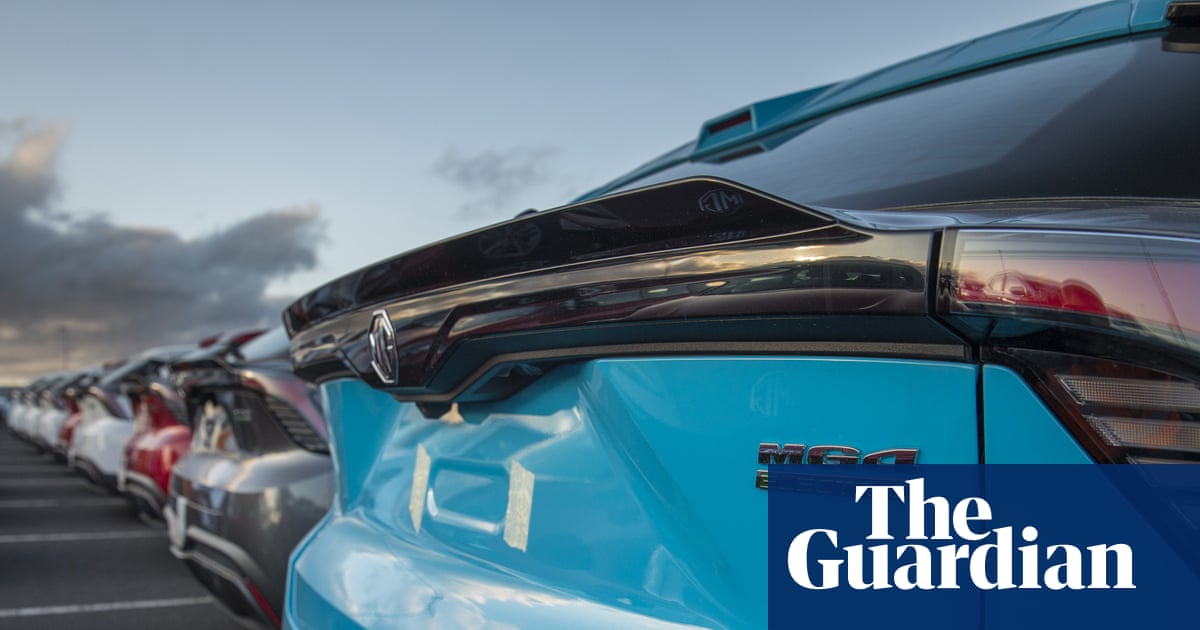
Electric vehicles are not travelling as far as their manufacturers promise, with independent road tests showing all models analysed have failed to meet their advertised range.
One popular small car produced the worst EV result to date in the latest tests, pulling up more than 120km short of the distance printed on its sticker. At the other end of the scale, Tesla’s latest Model Y SUV was only a few kilometres short of its claim.
The Australian Automobile Association released the findings on Thursday with another four electric car road trials held as part of its $14m Real-World Testing Program.
Sign up: AU Breaking News email
The results add to a previous round of electric vehicle examinations, in which all five models failed to meet their promised range, and after tests of 131 internal combustion and hybrid vehicles found that 76% consumed more fuel than advertised.
The association tests vehicles on a 93km track in and around Geelong, Victoria, on urban and rural roads, as well as motorways.
US car maker Tesla emerged with the best result from all electric car tests to date. Its Model Y SUV fell 16km short of its claimed range of 466km on a single charge.
By contrast, the MG4 electric hatchback produced the worst result so far, missing its 405km goal by 124km – a shortfall of 31%.
The Kia EV3 missed its mark by 11% or 67km, and the Smart #1 electric car stopped short by 13% or 53km.
Comparing the real-world range of electric cars to their laboratory results would be vital for motorists, association managing director Michael Bradley said, as it would help them reach decisions and set expectations.
“These results give consumers an independent indication of real-world battery range, which means they now know which cars perform as advertised and which do not,” he said.
skip past newsletter promotion
after newsletter promotion
“Giving consumers improved information about real-world driving range means buyers can worry less about running out of charge and make the switch to EVs with confidence.”
The association’s vehicle-testing program, funded by the federal government and launched in 2023, has tested 140 vehicles out of a target of 200, and has found most consume more energy or fuel than promised.
The Australian testing program was introduced following a 2015 Volkswagen scandal in which the European automaker was discovered using software to alter vehicle emissions during laboratory tests.
Boeing Elects Bradley D. Tilden to Board of Directors
– Tilden, former chairman, president and CEO of Alaska Air Group, will join Safety and Finance committees
ARLINGTON, Va., Dec. 3, 2025 /PRNewswire/ — The Boeing Company (NYSE: BA) today announced that its Board of Directors has elected Bradley D. Tilden as its newest member, effective Dec. 3, 2025. Tilden will join the Aerospace Safety and Finance committees.
Tilden, 64, previously served as chairman, president and CEO of Alaska Air Group, Inc., the parent company of Alaska Airlines and Hawaiian Airlines, as well as regional airline Horizon Air.
“Brad brings a distinct customer perspective, proven leadership in the airline industry, and more than three decades of aviation experience,” said Boeing Board Chair Steve Mollenkopf. “His experience in safety management systems and financial expertise will be invaluable to our Board as we continue to make progress in the company’s recovery.”
In his 31-year tenure at Alaska Air Group, Tilden held several senior leadership roles, including CFO and then president of Alaska Airlines. Beginning in 2012, he began serving as President and CEO of Alaska Air Group, and was named executive chairman in 2021.
The 12th member of the board, Tilden will be the 10th new director added since 2019, as part of the board’s refreshment efforts. These directors collectively bring significant experience in aerospace, safety, engineering, manufacturing, cyber, artificial intelligence, software, risk oversight, audit, supply chain management, sustainability and finance, as well as the perspective of customers, suppliers and pilots.
A leading global aerospace company and top U.S. exporter, Boeing develops, manufactures and services commercial airplanes, defense products and space systems for customers in more than 150 countries. Our U.S. and global workforce and supplier base drive innovation, economic opportunity, sustainability and community impact. Boeing is committed to fostering a culture based on our core values of safety, quality and integrity.
Roula Khalaf, Editor of the FT, selects her favourite stories in this weekly newsletter.
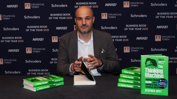
Stephen Witt’s The Thinking Machine, about the rise of Nvidia and its hard-driving leader Jensen Huang, has won the 2025 Financial Times and Schroders Business Book of the Year Award.
It is the second year in succession that the £30,000 award has gone to a book about the rapid spread of generative artificial intelligence. Last year’s winner, Supremacy by Parmy Olson, examined the rivalry between OpenAI and DeepMind.
Richard Oldfield, chief executive of asset management group Schroders, presented Witt with the prize at a dinner in London on Wednesday, mentioning how the judges praised The Thinking Machine’s “unique insights” into the success of Huang and Nvidia. In October, the chipmaker became the first company to surpass a market value of $5tn.
Roula Khalaf, FT editor and chair of judges, called the book “a fascinating account of the making of one of the most consequential companies of our times”.
Television producer and investigative journalist Witt was shortlisted for the FT award in 2015 for his book How Music Got Free, the story of how piracy and peer-to-peer sharing disrupted the recorded music industry.
The judges also praised the five other shortlisted titles, each of which is awarded £10,000, for the way in which they summed up critical issues facing business and the world, including US-China rivalry and the quest for growth and prosperity.
The award, which is also supported by FT owner Nikkei, is now in its 21st year. Previous winners include Amy Edmondson in 2023 for Right Kind of Wrong, about how to learn from failure and take better risks, and Chris Miller’s Chip War in 2022, about the global battle for semiconductor supremacy.
The other 2025 finalists were: House of Huawei by Eva Dou, which investigates the rise of the Chinese technology company and its founder; Chokepoints by Edward Fishman, about the use of economic sanctions; How Progress Ends by Carl Benedikt Frey, on what decides the destiny of civilisations; Abundance by Ezra Klein and Derek Thompson, about the growth dilemma facing the US; and Breakneck by Dan Wang, contrasting the US and its arch-rival China.
The other judges of this year’s award were Mimi Alemayehou, founder and managing partner, Semai Ventures; Daisuke Arakawa, senior managing director for global business, Nikkei; Mitchell Baker, founder, former CEO and executive chair, Mozilla; entrepreneur, angel investor and board leader Sherry Coutu; Mohamed El-Erian, professor of practice at the Wharton School, University of Pennsylvania, chief economic adviser, Allianz, and chair, Gramercy Funds Management; James Kondo, chair, International House of Japan; Adam Osborn, head of research, Asia ex Japan equities, Schroders; Randall Kroszner, economics professor at University of Chicago’s Booth School of Business; Nicolai Tangen, CEO, Norges Bank Investment Management; and Shriti Vadera, chair of Prudential and the Royal Shakespeare Company.
For more on this year’s award and previous winners, visit www.ft.com/bookaward
President Donald Trump on Wednesday said his administration would “reset” fuel efficiency standards for passenger cars in an effort to put a lid on rising auto prices, as the administration battles inflation and an affordability crisis.
The previous rules, which sought to lower carbon emissions, “put tremendous upward pressure on car prices,” Trump said in the Oval Office.
The president is under political pressure to address affordability concerns after Democrats swept major races last month, fueled by voters’ frustration with rising prices.
Overall inflation, as measured by the consumer price index, has risen every month since Trump announced sweeping tariffs on imported goods, including automobiles and car parts, among other items. Food prices have also been rising this year. In early November, the White House announced cuts to dozens of tariffs in a move aimed at cutting food prices.
The average new vehicle price in October surged to an all-time high, above $50,000 for the first time ever, according to Kelley Blue Book. However, KBB said that “despite higher prices, retail sales continue to maintain a healthy pace.”
“The $20,000-vehicle is now mostly extinct, and many price-conscious buyers are sidelined or cruising in the used-vehicle market,” Cox Automotive analyst Erin Keating said in October.
The Department of Transportation says the proposal will “save the American people $109 billion” or $1,000 on the average cost of a new vehicle, but it’s unclear how fast prices could fall. The updated standards still must go through a formal rulemaking process before being finalized, likely in 2026.
The proposed change “will also revive the beating heart of American manufacturing and unshackle the nation’s automotive industry,” the department and the National Highway Traffic Safety Administration said.
It would also roll back efficiency mandates raised by the Biden administration.
“The announcement today is a shift in long-term fuel economy targets for model year 2031 vehicles,” said Mark Schirmer, Cox Automotive’s director of industry insights communications.
“Those targets are being lowered, which may change automaker long-term strategy and product development plans and pricing, but will have little impact on prices near term,” he said.
The administration also said it would reclassify crossover vehicles and small SUVs as passenger automobiles instead of light trucks, removing what it called a “market distortion that existed for decades.”
President Donald Trump alongside lawmakers and automotive executives in the Oval Office.Andrew Caballero-Reyonds / AFP via Getty Images
Trump was joined at the White House for the announcement by executives from Detroit’s “Big Three” — Stellantis CEO Antonio Filosa, Ford Motor Company CEO Jim Farley and John Urbanic, executive plant director of General Motors’ Orion assembly factory in Michigan.
Stellantis is the European parent company of the Chrysler, Dodge, Jeep and Ram car brands.
In statements, all three of the companies praised the move. Stellantis said it would “re-align … standards with real world market conditions,” while Ford said “we can make real progress on carbon emissions and energy efficiency while still giving customers choice and affordability.”
“This is a win for customers and common sense,” Ford’s Farley added.
General Motors said it has “long advocated for one national standard that upholds customer choice and provides the auto industry long-term stability.”
The Chevy and Cadillac maker added that it remains “committed to offering the best and broadest portfolio of electric and gas-powered vehicles on the market.”
Shares of Ford and GM stock closed about 1% higher Wednesday. Stellantis’ stock jumped 4.7%.