
For many years, nuclear physicists believed that “Islands of Inversion” were found mainly in isotopes packed with extra neutrons. These unusual regions of the nuclear chart are places where the normal structure of atomic nuclei suddenly stops…
Category: 7. Science
-
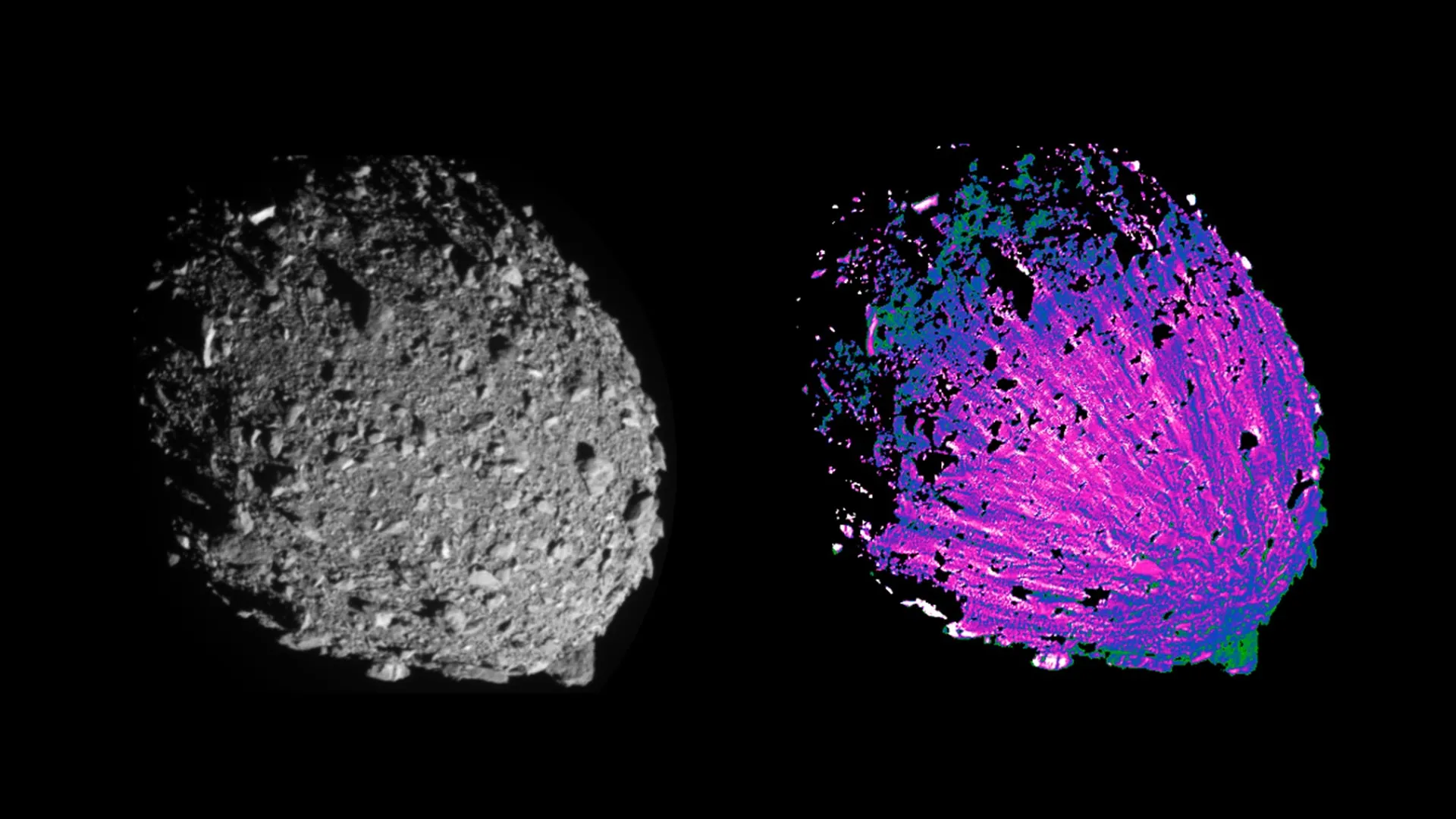
NASA DART mission reveals asteroids throw “cosmic snowballs” at each other
Roughly 15% of asteroids that pass near Earth have a smaller companion orbiting them. These paired objects are known as binary asteroid systems, and they are surprisingly common in our region of the solar system.
A research team led by the…
Continue Reading
-
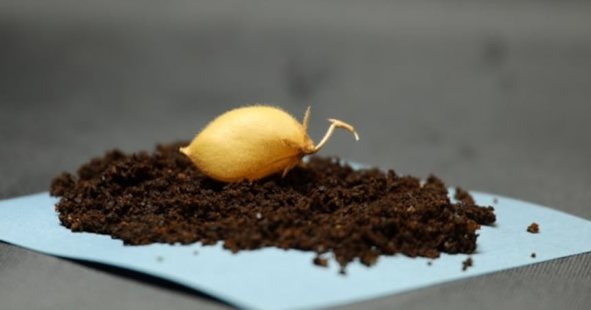
Chickpeas Grown in Simulated Lunar Soil – 조선일보
- Chickpeas Grown in Simulated Lunar Soil 조선일보
- Bioremediation of lunar regolith simulant through mycorrhizal fungi and plant symbioses enables chickpea to seed Nature
- Can we grow life on Mars? Experiments show potential in simulated…
Continue Reading
-
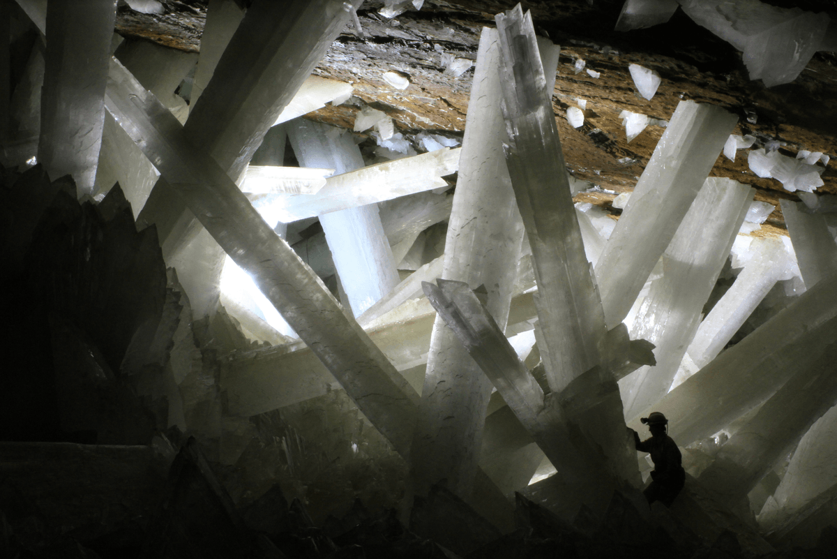
It’s a staggering 300 metres underground, features amazing 11-metre-tall crystals – and has a deadly 90% humidity level
The aptly named Cave of Crystals, in Chihuahua, Mexico, is buried around 300 metres underground and contains giant gypsum crystals up to 11 metres long.
Some are big enough to walk on and are so impressive they earned the cave its alternative…
Continue Reading
-
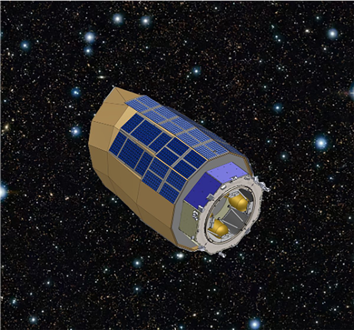
Ex-Google boss may launch a bigger-than-Hubble space telescope within three years
When Yerkes Observatory opened in Wisconsin in 1897, it was a wonder.
Alongside the great one-metre (40-inch) telescope – the largest refractor ever built – the lavish facilities included the novelty of chemical and physical laboratories to…
Continue Reading
-
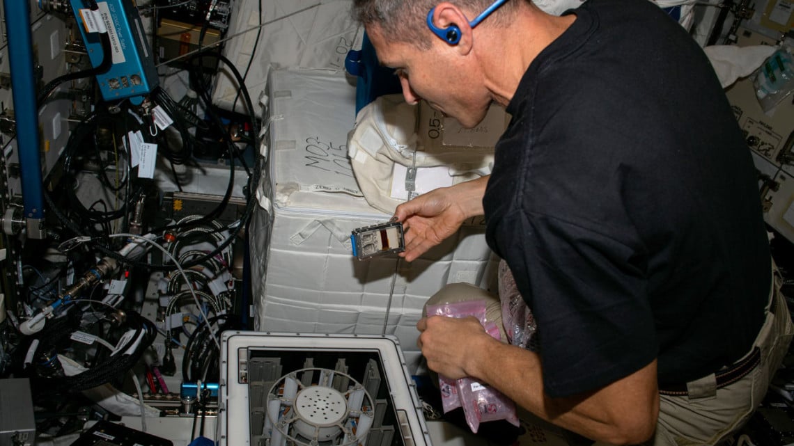
Astronauts Use Bacteria and Fungi to Harvest Metals in Space
It’s a well-known fact that if humanity wishes to explore deep space and to live and work on other planets, we need to bring Earth’s environment with us. This includes life support systems that leverage biological processes – aka.
Continue Reading
-
High-resolution, high-throughput detection of hidden antibiotic resistance with the dilution-and-delay (DnD) susceptibility assay
Martens, E. & Demain, A. L. The antibiotic resistance crisis, with a focus on the United States. J. Antibiot. 70, 520 (2017).
Currie, C. J. et al. Antibiotic treatment failure in four common…
Continue Reading
-
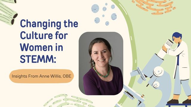
Anne Willis On RNA Research And Women In STEMM
Professor Anne Willis is director of the Medical Research Council Toxicology Unit and professor of Toxicology at the University of Cambridge. She obtained her PhD from Imperial College, London, working with Tomas Lindahl at the ICRF Clare…
Continue Reading
-
Molecular identification of bat fly species and associated Bartonella bacteria from Lopburi and Sa Kaeo Provinces in Thailand
Kunz, T. H., Braunde de Torrez, E., Bauer, D., Lobova, T. & Fleming, T. H. Ecosystem services provided by bats. Ann. N Y Acad. Sci. 1223, 1–38. https://doi.org/10.1111/j.1749-6632.2011.06004.x (2011).
Continue Reading