Gong, R., Xu, L., Wang, D., Li, H. & Xu, J. Water quality modeling for a typical urban lake based on the EFDC model. Environ. Model. Assess. 21, 643–655. https://doi.org/10.1007/s10666-016-9519-1 (2016).
Category: 7. Science
-
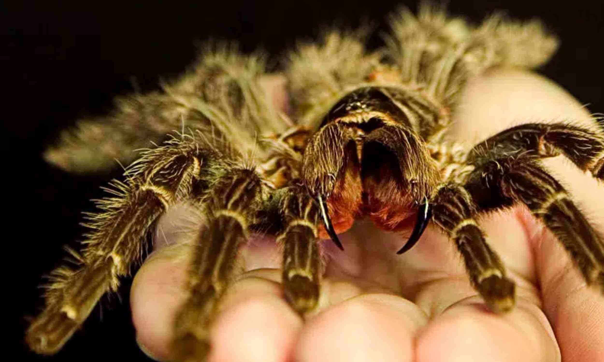
Giant spider returns after successful nature reclamation project
Scientists have confirmed that a rare burrowing spider known as the northern tarantula now lives in restored grassland where farm fields once covered the ground.
Its return shows that rebuilt meadows can quickly create the warm soil, steady…
Continue Reading
-

The Moon is collecting a massive chemical archive of planet Earth
Earth’s atmosphere may feel permanent, but it is slowly leaking into space. New research suggests some of that lost air does not disappear.
Instead, it drifts outward and settles onto the Moon, quietly accumulating in lunar soil over billions…
Continue Reading
-
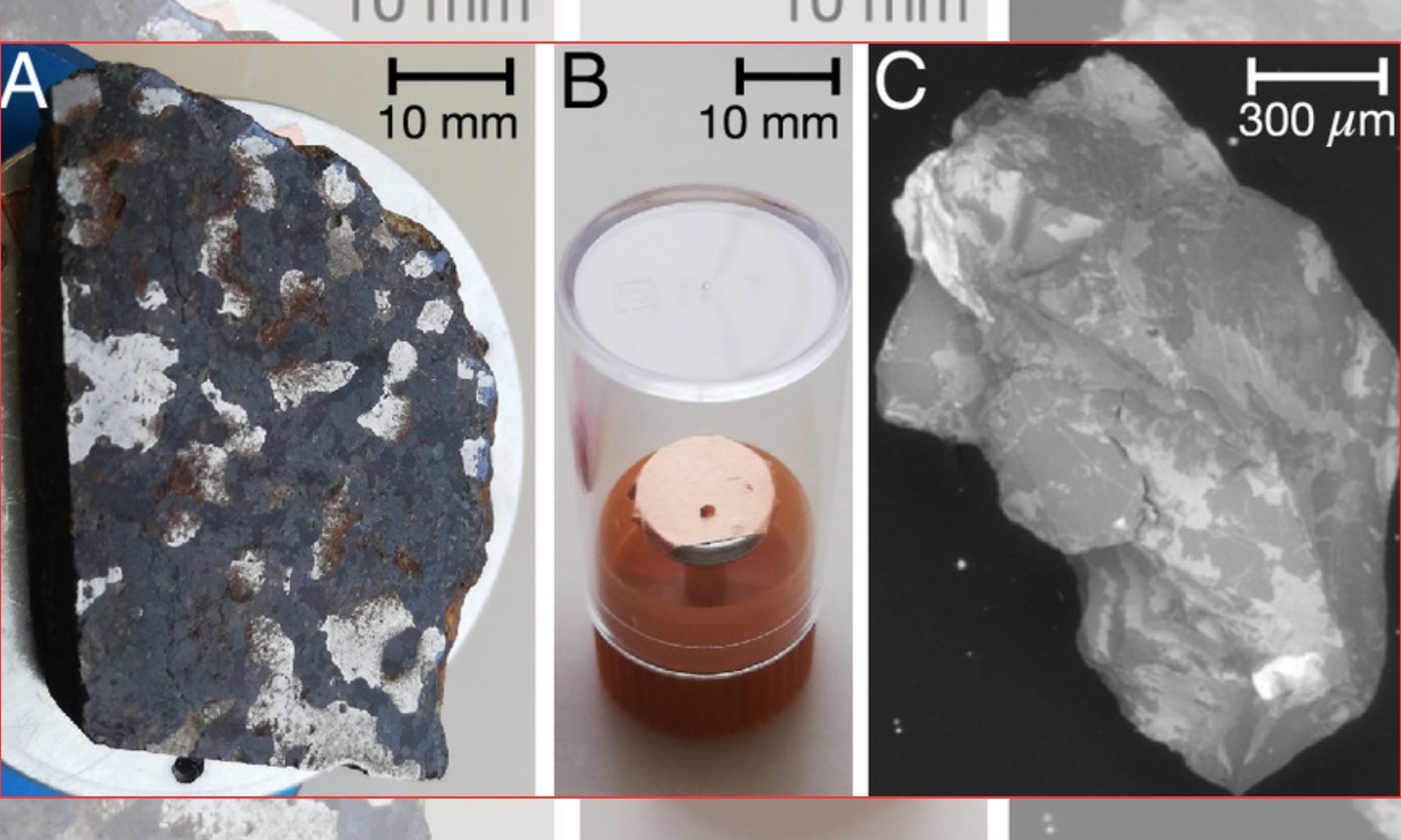
Meteorite from 1724 challenges the fundamental rules of physics
A fragment of a centuries-old meteorite has revealed a form of solid silica that carries heat at nearly the same rate across a wide span of temperatures.
That stability challenges one of the simplest assumptions about how solids behave, blurring…
Continue Reading
-
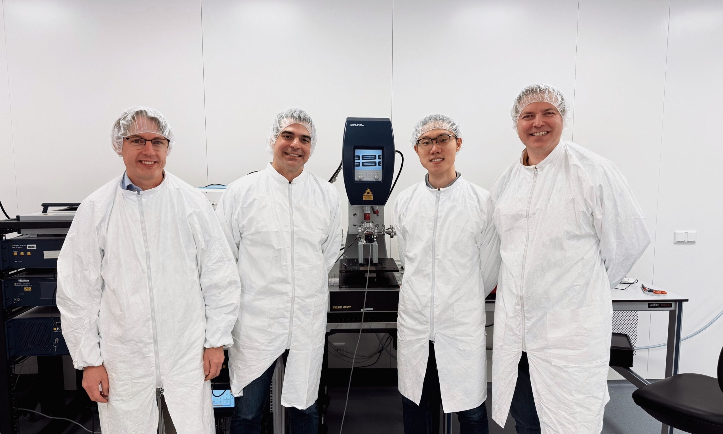
Nanostring creation could increase the sensitivity of future sensors
A tiny on-chip string has been shown to pass energy from its simplest vibration into several higher ones.
Instead of leaking straight into the environment, that energy stayed inside long enough to create several signals from one device.
Cascade…
Continue Reading
-
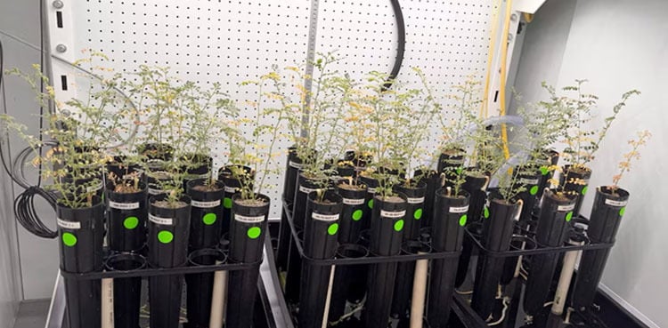
Scientists grow chickpeas in ‘moon dirt’
If the idea of lunar hummus seems far-fetched, think again. Scientists working to cultivate the field of extraterrestrial agriculture have grown chickpeas in dirt made mostly of simulated lunar soil, a step toward enabling astronauts on…
Continue Reading
-
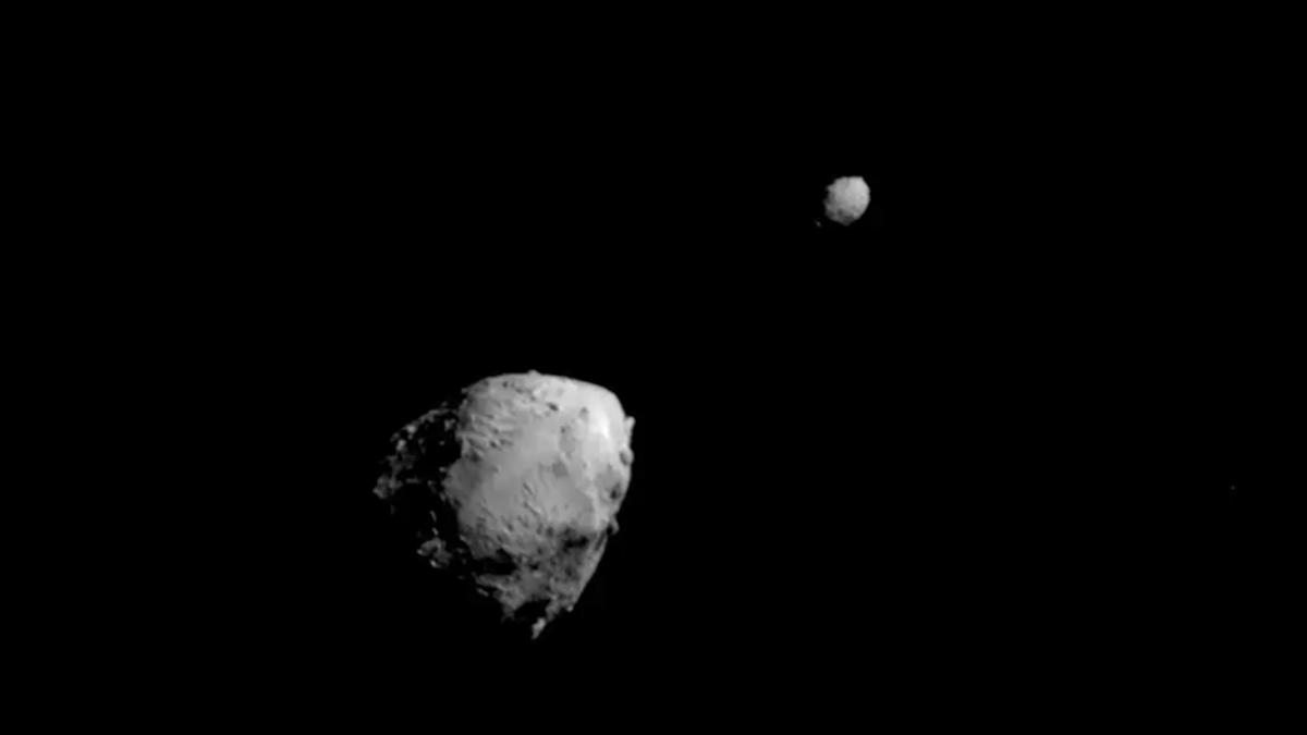
NASA’s DART spacecraft changed a binary asteroid’s orbit around the sun, in a first for a human-made object
When NASA crashed a spacecraft into the asteroid moonlet Dimorphos in 2022, it altered both Dimorphos’ orbit around its parent asteroid, Didymos, and the two objects’ orbit around the sun, according to new research. NASA’s Jet Propulsion…
Continue Reading
-
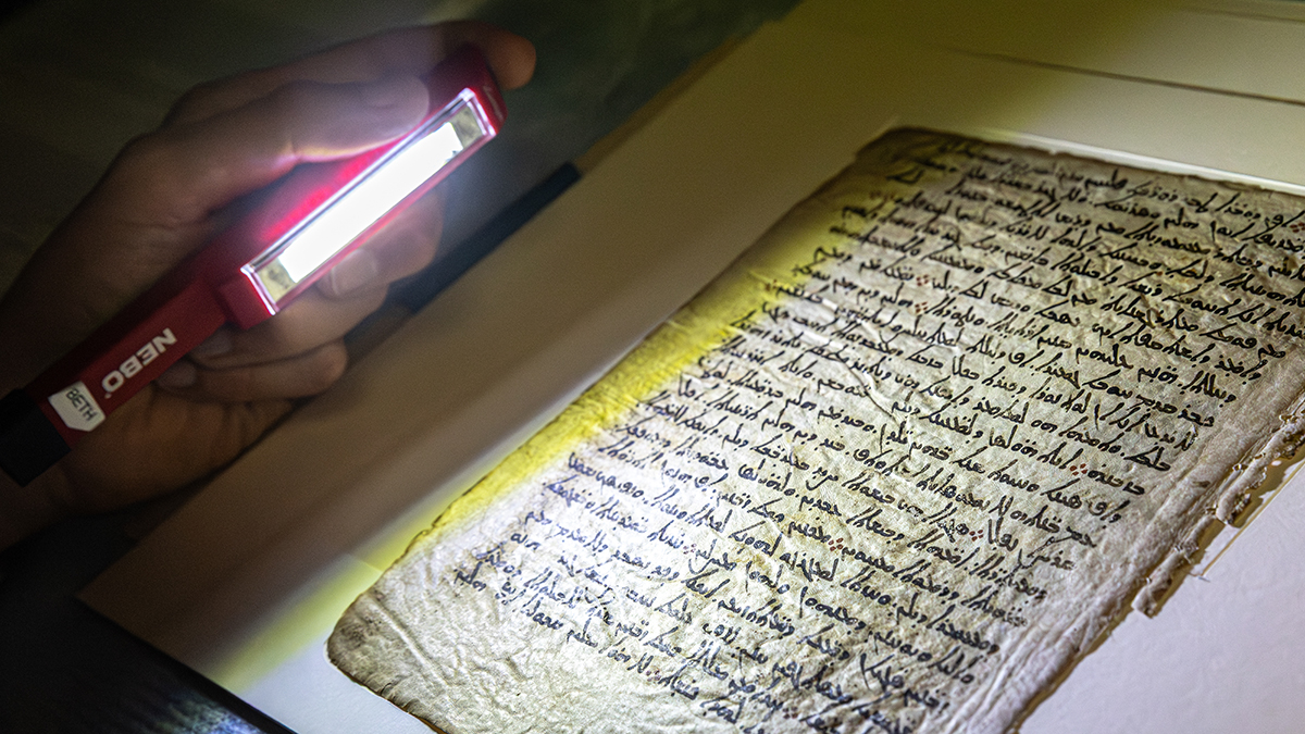
Scientists Reveal The Oldest Map of The Night Sky Ever Made : ScienceAlert
Researchers are painstakingly reconstructing the oldest-known map of the night sky – previously thought lost forever – by X-raying parchment that contains the star catalog hidden beneath other text.
The map of the cosmos is thought to be…
Continue Reading
-
The chromosome-scale genome assembly and annotation of Rosa bracteata (Macartney Rose)
Ku, T. R. K. Rosa (Rosaceae). In Flora of China 9 (eds Wu, Z. Y. & Raven, P. H.) (Missouri Botanical Garden, 2003).
Luo, L. Genus Rosa L. in China (China Forestry Publishing House, 2024).
Cheng, B. et al. Phenotypic and genomic signatures across…
Continue Reading