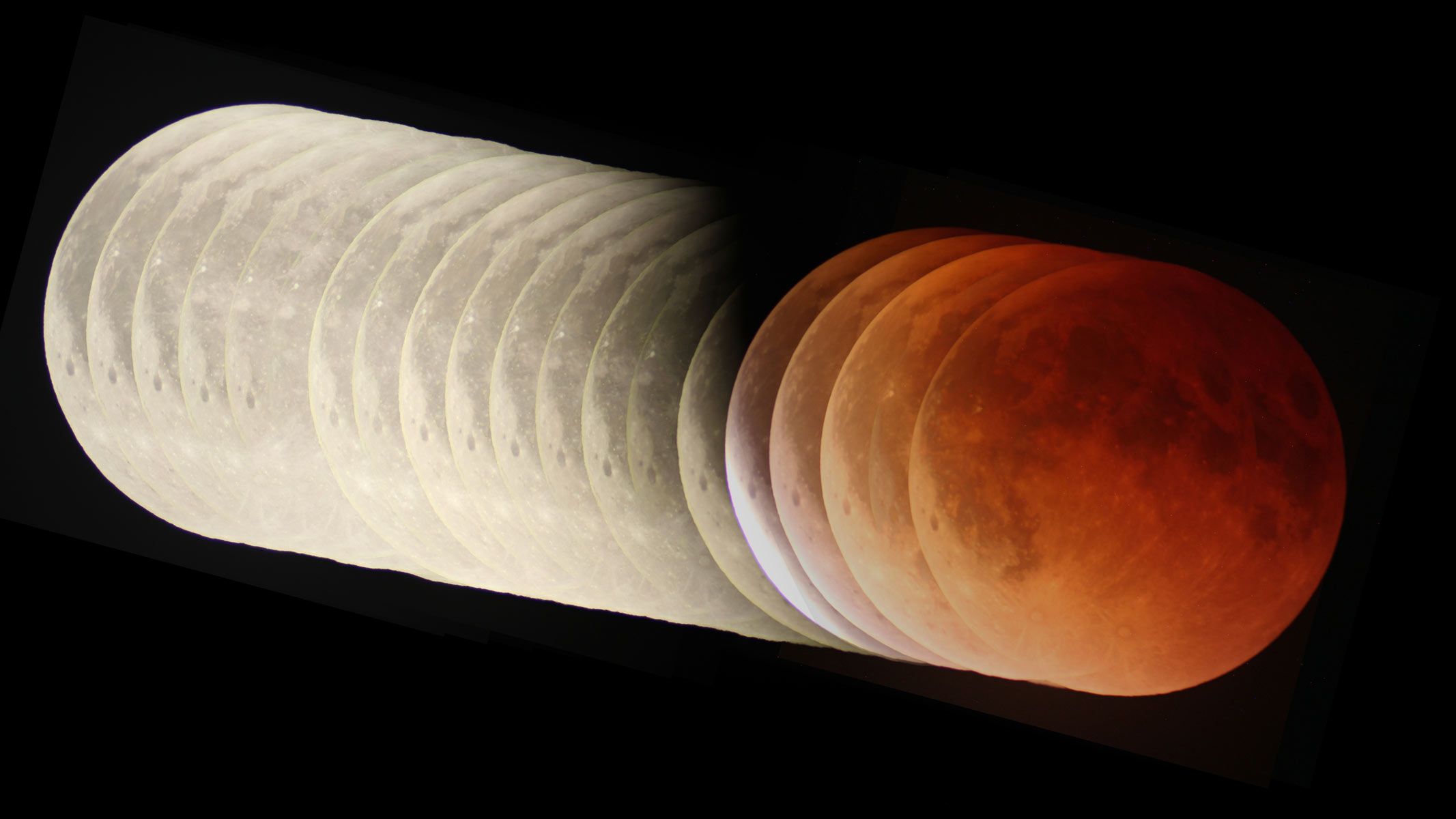
On March 3, 2026, the full Worm Moon will slip into Earth’s shadow and turn a strange copper-reddish color for 58 minutes. To the naked eye, it will be a beautiful sight, with the full moon’s light extinguished as a “blood moon” sits in a…
Category: 7. Science
-
What to expect during the ‘blood moon’ total lunar eclipse tonight — Key phases explained
On March 3, billions of people across the Americas, Asia and Oceania will witness a blood moon total lunar eclipse as the sun, Earth and moon align, laying bare the orbital mechanics of the solar system in spectacular fashion.
The eclipse occurs…
Continue Reading
-
Tuesday’s ‘Blood Moon’ Eclipse: Exact Times For Every U.S. State – Forbes
- Tuesday’s ‘Blood Moon’ Eclipse: Exact Times For Every U.S. State Forbes
- Where to see the total lunar eclipse in the early hours of March 3 Space
- How and when to see the total lunar eclipse on March 3 CBC
- Last total lunar eclipse until late…
Continue Reading
-

Early plant expansion timeline revised
Early land plants may have begun reshaping Earth”s surface much earlier than previously thought — pushing the timeline back by about 30 million years, according to a new study.
The findings, resulting from research by…
Continue Reading
-
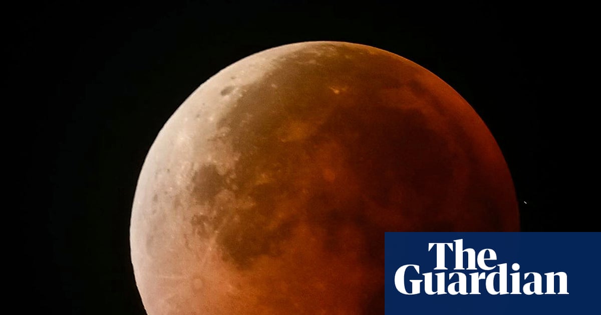
Rare ‘blood moon’ total lunar eclipse to loom over North America, Australia and New Zealand | Science
North America, Australia and New Zealand will be treated to a rare total lunar eclipse on Tuesday known as a “blood moon”.
As the full moon dips into the planet’s shadow it will change colour to a “deep and coppery red”, says…
Continue Reading
-
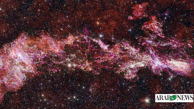
Vast web of cold gas observed at the heart of the Milky Way – Arab News PK
- Vast web of cold gas observed at the heart of the Milky Way Arab News PK
- New image reveals secrets of Milky Way galaxy in stunning detail The Guardian
- Mapping the Cosmic Heart: A New View into Our Galaxy’s Core Devdiscourse
- Central Molecular…
Continue Reading
-
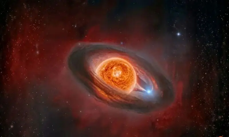
Dramatic changes observed in one of universe’s biggest stars – Life & Style
The largest stars in the universe live the life of a rock star — they are born brilliant, live fast and die young. If that is the case, the one named WOH G64 might be considered the stellar equivalent of Jimi Hendrix.
WOH G64, which is 28 times…
Continue Reading
-

SpaceX launches 25 Starlink Satellites on its Falcon 9 booster from the West Coast
SpaceX is all set to launch a Falcon 9 rocket early Sunday…
Continue Reading
-
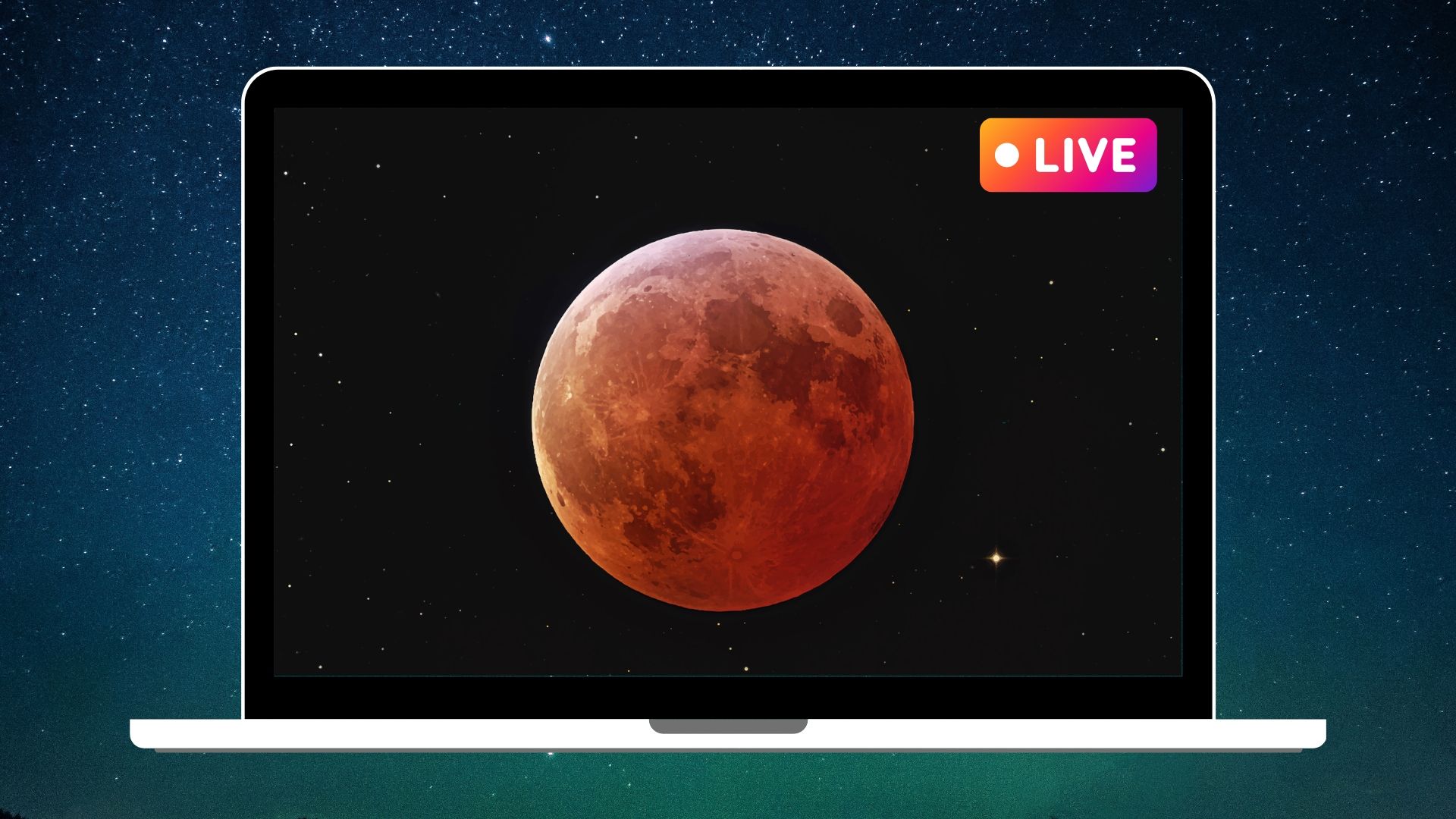
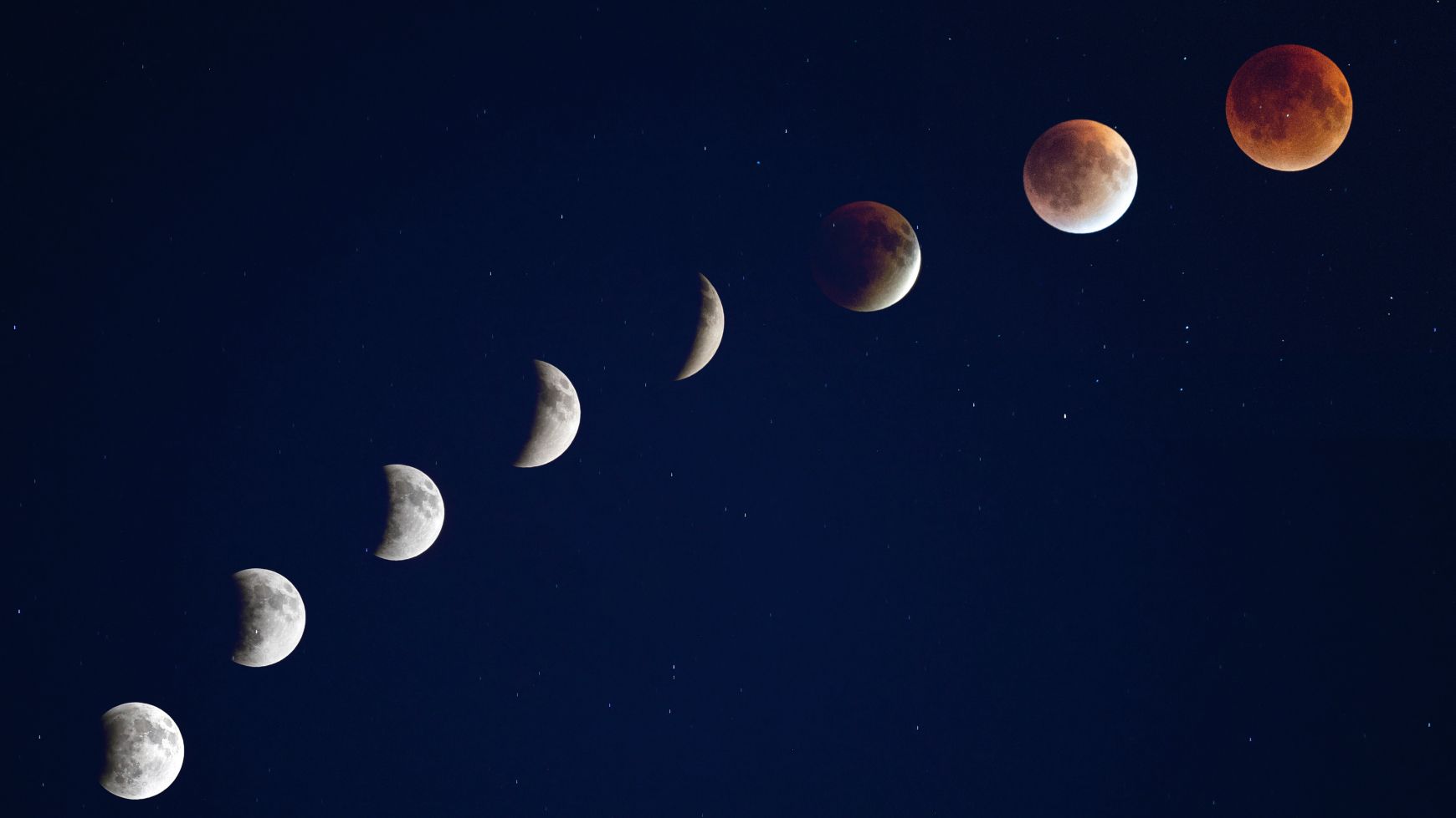
Watch the ‘blood moon’ total lunar eclipse on March 3 with these free livestreams
Stargazers across the U.S. will be treated to a dramatic orbital display in the early hours of March 3, as Earth’s shadow falls across its natural satellite, giving rise to a“blood moon” total lunar eclipse.
Over 3.3 billion people across the…
Continue Reading
-

New observatory sends 800,000 asteroid alerts in one night
The Vera C. Rubin Observatory has officially activated its automated alert system, to…
Continue Reading