
Scientists at Kyoto University have developed a theoretical model examining whether disturbances in the ionosphere could apply electrostatic forces deep within the Earth’s crust. Under certain conditions, these forces might contribute to the…
Category: 7. Science
-

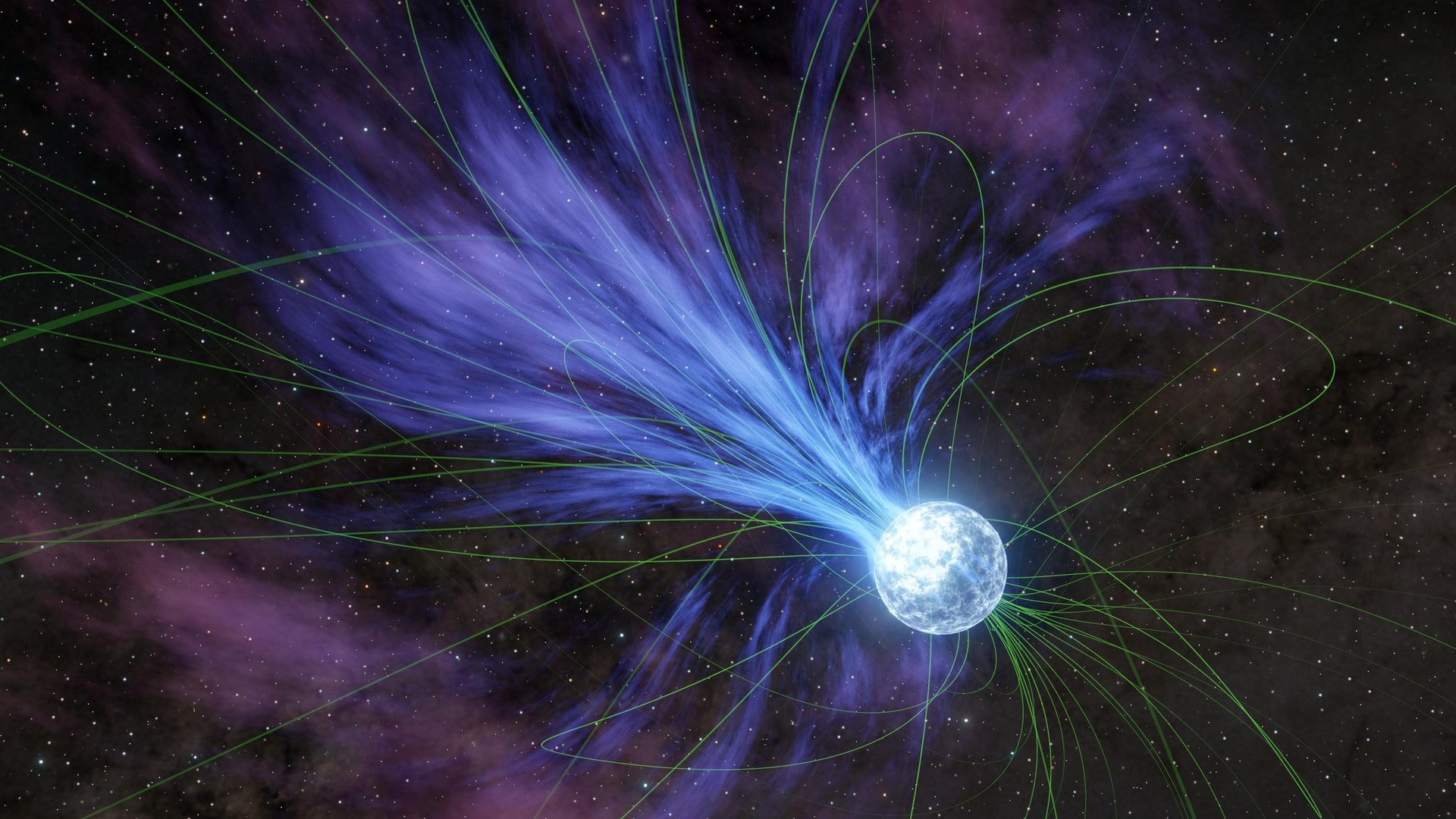
Starlight warped in the fabric of spacetime could help us find hidden black holes dancing together
Two supermassive black holes on a dizzying death spiral could soon become visible to astronomers after researchers worked out how, while rotating around each other, these dark, massive behemoths could gravitationally lens the stars behind…
Continue Reading
-
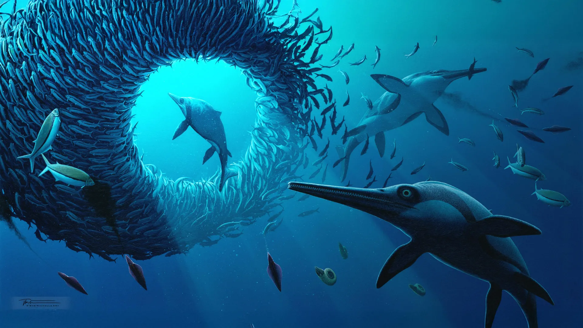
190-million-year-old “Sword Dragon” fossil rewrites ichthyosaur history
A remarkably complete skeleton uncovered along the UK’s Jurassic Coast has been identified as a previously unknown species of ichthyosaur — a group of prehistoric marine reptiles that once dominated the world’s oceans.
The dolphin-sized…
Continue Reading
-

Total lunar eclipse March 2026 — Live updates
Refresh
Who will be able to see the total lunar eclipse?
The ‘blood moon’ will be visible to skywatchers across western North America, Australia, New Zealand and eastern Asia, weather dependent. (Image credit:… Continue Reading
-
A “Cosmic Positioning System” in the Outer Solar System
There have been plenty of attempts to resolve the “Hubble Tension” in cosmology. This feature describes how one of the most important variables in cosmology, the expansion of the universe, takes on different values depending on how…
Continue Reading
-

Where to see the total lunar eclipse in the early hours of March 3
The first lunar eclipse of 2026 will transform the moon into a coppery red “blood moon” in the early hours of March 3 for skywatchers in North America.
The long-lasting and impressive blood moon on March 3 will be visible to billions within the…
Continue Reading
-
Scientists Discover DNA Is Already Organized Before Life Switches On – SciTechDaily
- Scientists Discover DNA Is Already Organized Before Life Switches On SciTechDaily
- Global reorganization of genome architecture at the transition to gametogenesis Nature
- New technology reveals hidden DNA scaffolding built before life ‘switches…
Continue Reading
-

SMILE spacecraft sets sail for French Guiana before landmark solar wind mission launch
image: ©aapsky | iStock A landmark European-Chinese space mission with strong British leadership is on its way to its launch site in South America
SMILE begins launch
The Solar Wind Magnetosphere Ionosphere Link Explorer…
Continue Reading
-

Plant Hormone Therapy Boost Global Food Security
Key takeaways
- Plants can defend against disease, but their growth is stunted when their immune systems are triggered. That’s a problem if the plant is raised for food.
- CSU researchers have discovered how to turn on a hormone that allows…
Continue Reading