This week’s science news was bursting with discoveries of archaeological treasures, starting with the revelation that a foundation stone for a Czech garden barn was actually a Bronze Age spearhead mold.
The mold, carved into ancient volcanic…
This week’s science news was bursting with discoveries of archaeological treasures, starting with the revelation that a foundation stone for a Czech garden barn was actually a Bronze Age spearhead mold.
The mold, carved into ancient volcanic…
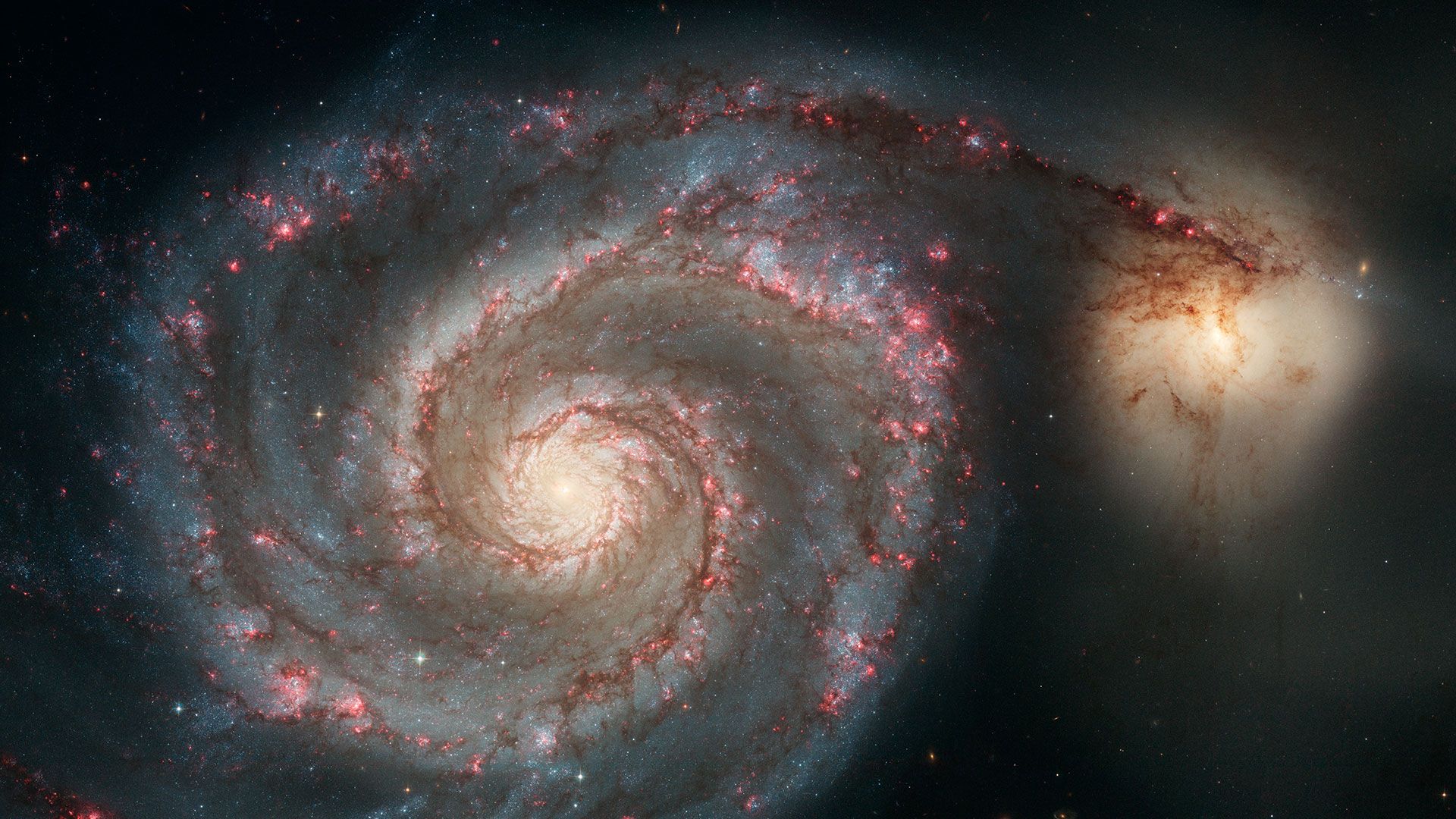
Spring is almost here, which means it’s galaxy season for amateur astronomers! Grab your telescope and join us as we highlight some of the most beautiful galactic targets visible in the spring night sky over the coming months.
Van de Peer, Y., Mizrachi, E. & Marchal, K. The evolutionary significance of polyploidy. Nat. Rev. Genet. 18, 411–424. https://doi.org/10.1038/nrg.2017.26 (2017).
Gillard, G. B. et al….

You might not be aware of this, but the Earth actually casts a huge shadow into space, and…
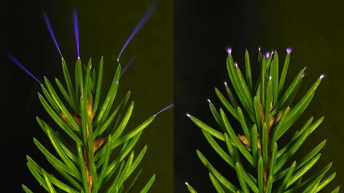
This week in science: The ESA is investigating a fireball that streaked across the skies in Europe and damaged a house in Germany; scientists detect a spooky glow coming from trees during thunderstorms; bumblebee queens found to be able to…

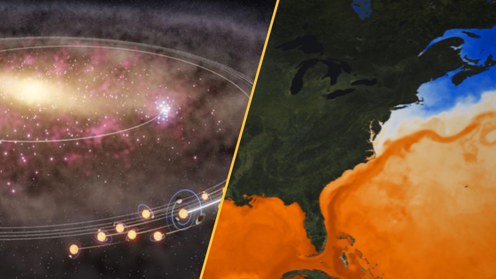
When we think of evolution, the gradual evolutionary change comes to mind: dinosaurs turning into birds, ancient forests transforming into the world around us. But therefore, all these upheavals hide a more subtle story, one that occurs at the…
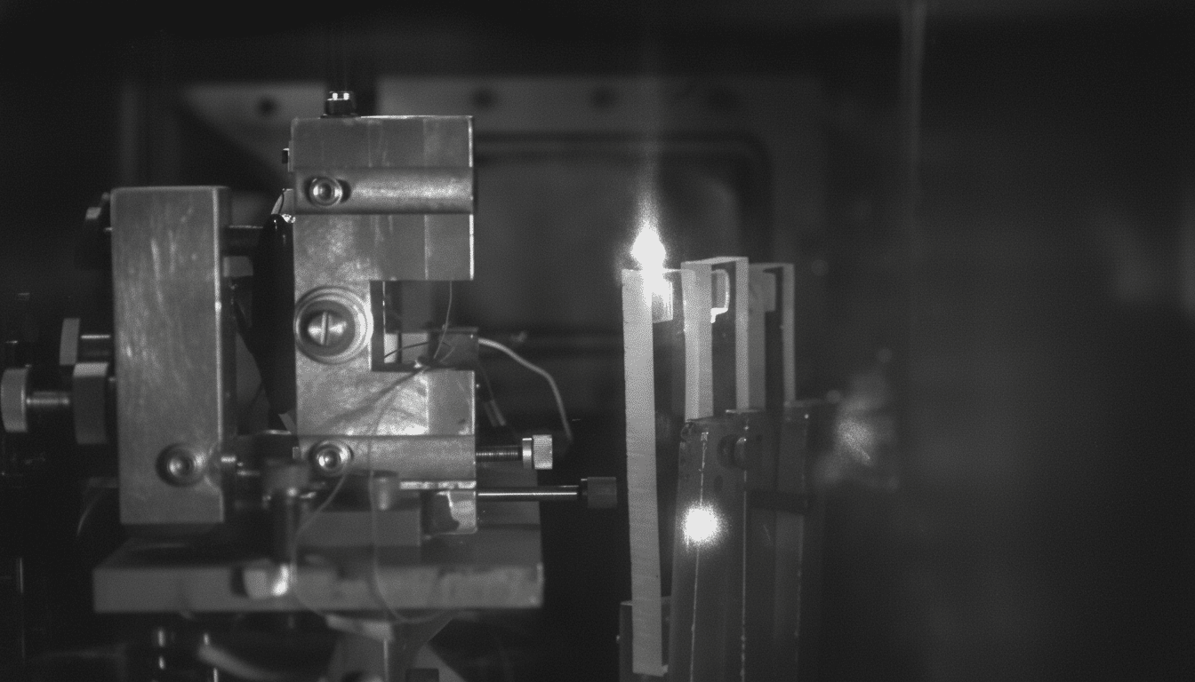
A striking set of impact experiments has strengthened the case that tiny life could hitchhike between worlds inside rocks blasted off a planet. In a Johns Hopkins University study funded by NASA and published in PNAS Nexus, researchers showed…
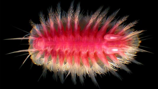
Rattail fish can grow up to a metre in length (3.2ft) and live at depths of up to 4,000m (13,100ft). Down there, far beyond the reach of the sun, the only light is made by living organisms – and the rattail’s big blue eyes can glimpse even the…
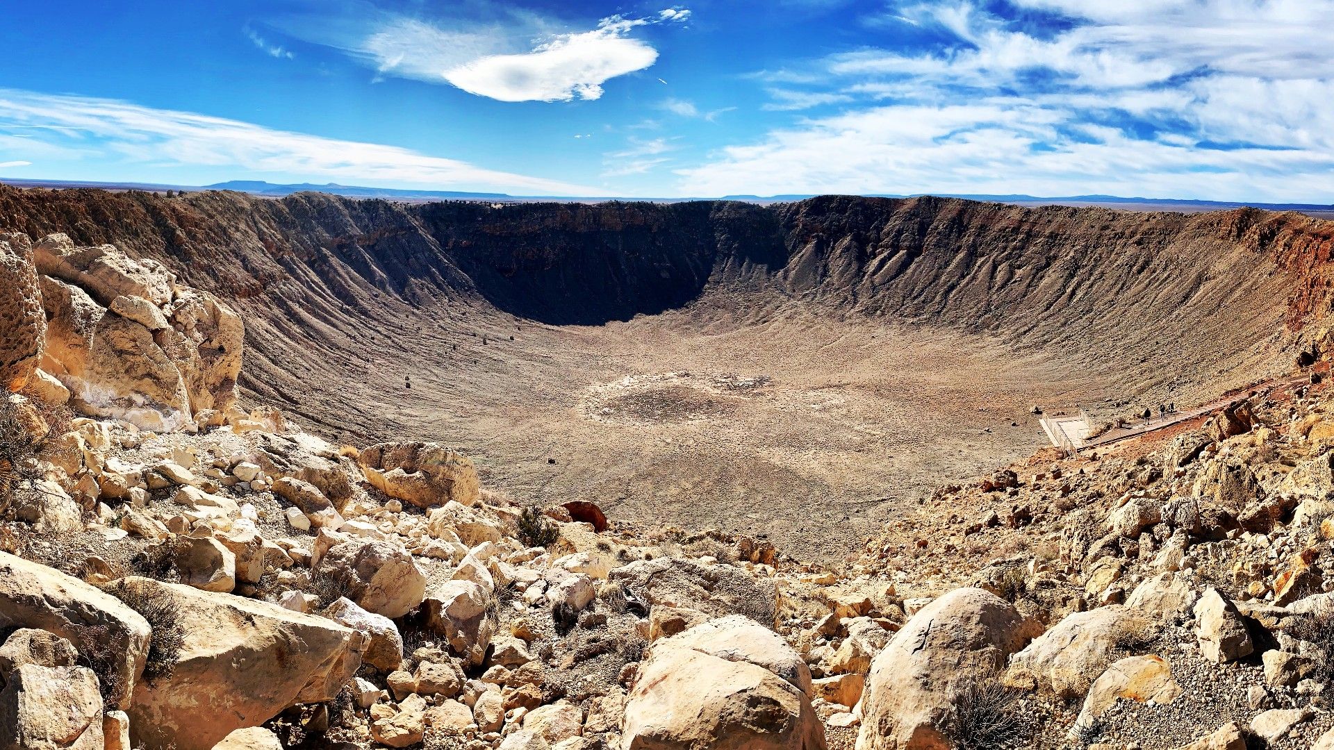
Arizona’s Meteor Crater and other scars leftover from collisions with space rocks continue to serve up their secrets.
Meteor Crater formed some 50,000 years ago. It represents the best preserved meteor impact site in the world, measuring some…
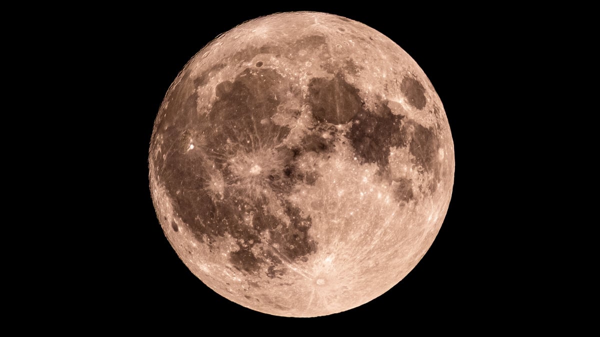
With the New Moon just a few days away, the Moon is shrinking into a thin crescent, with its lit surface fading more each night. For now, there’s still a small bit of its surface…