Brazilian scientists in a recent breakthrough have revealed…
Category: 7. Science
-
‘Unprecedented in the past 3.6 million years’: How human-made climate change is making days longer – Euronews.com
- ‘Unprecedented in the past 3.6 million years’: How human-made climate change is making days longer Euronews.com
- Human Activity Is Actually Making Earth’s Days Longer ZME Science
- Scientists say length of days on Earth is increasing at an…
Continue Reading
-
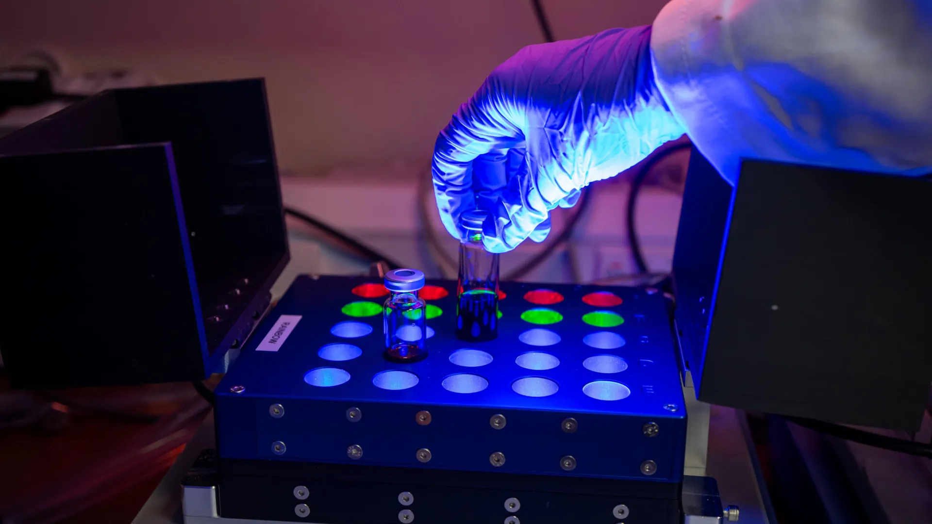
A lab mistake at Cambridge reveals a powerful new way to modify drug molecules
Researchers at the University of Cambridge have created a new technique that uses light instead of toxic chemicals to change complex drug molecules. The discovery could speed up drug development and make the process of designing medicines more…
Continue Reading
-

Chinese astronomers discover star formation in high-velocity cloud
Chinese astronomers have found a pair of young star clusters formed within a circumgalactic high-velocity cloud on the outskirts of the Milky Way—the first direct evidence of star formation in such an…
Continue Reading
-

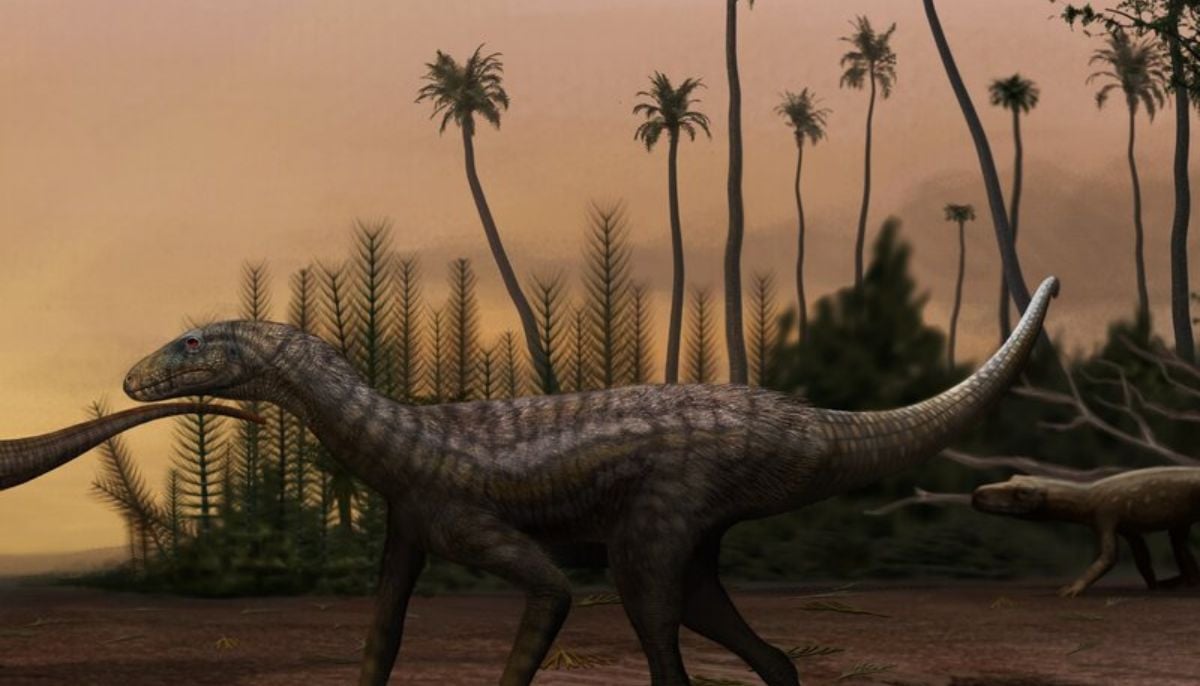
Scientists discover ancient DNA “switches” hidden in plants for 400 million years
Most people are familiar with the idea of deep space, but scientists also study something called deep time. Advances in genetics now allow researchers to trace biological changes far deeper into the past than previously possible. Even with these…
Continue Reading
-
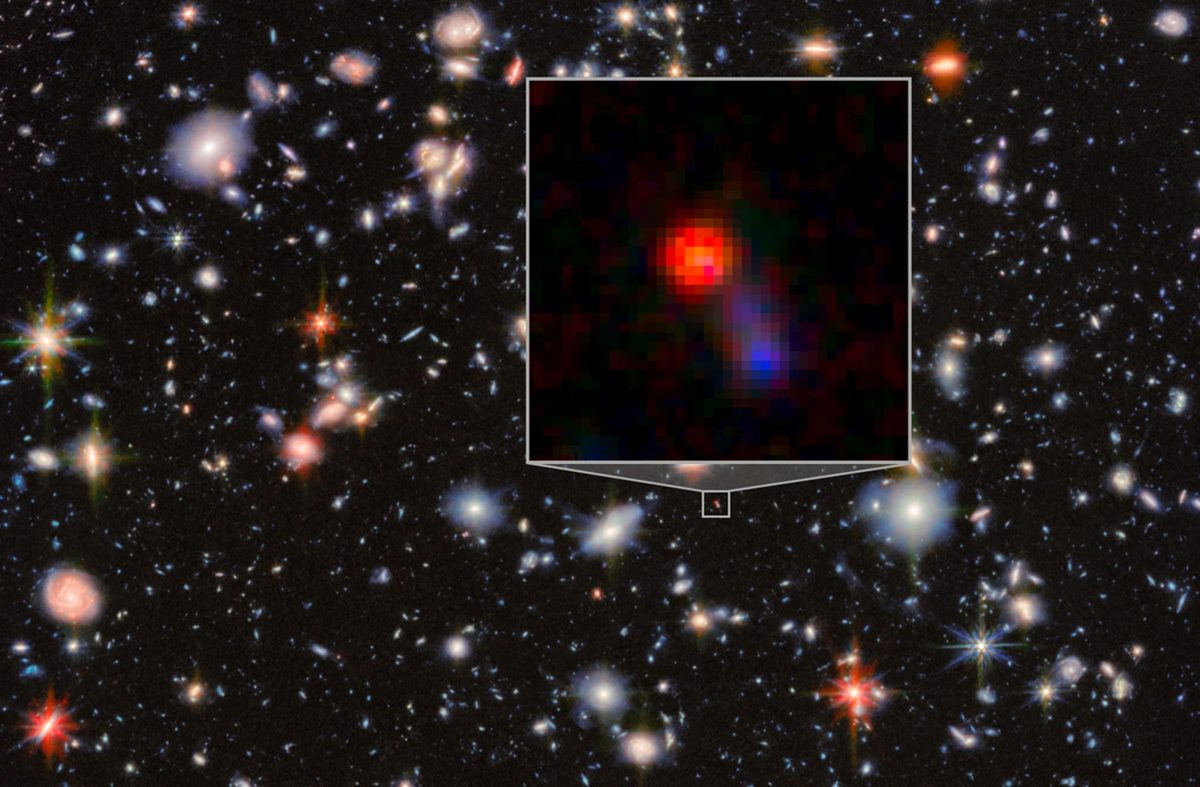
A scientist looked at ‘little red dots’ in the early Universe and found a black hole that shouldn’t exist
There’s something strange going on in the early Universe.
The James Webb Space Telescope has peered so deep into the cosmos, it’s effectively been able to look back in time to show what the Universe was like just after the Big Bang.
It’s found…
Continue Reading
-
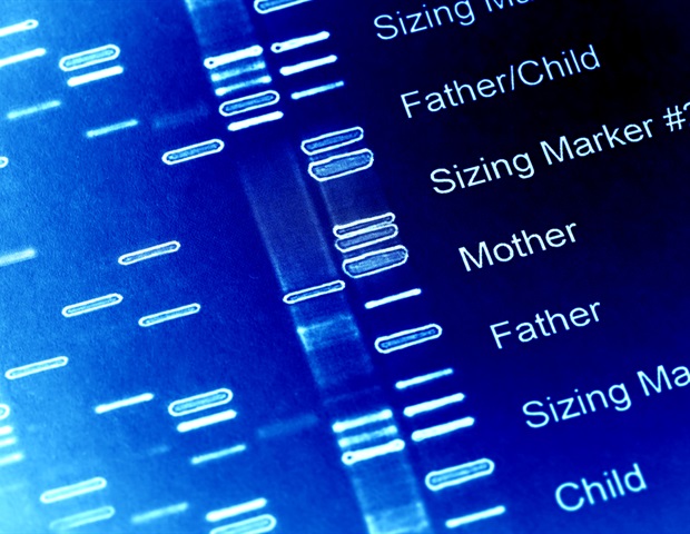
Selfish chromosomes hijack Overdrive gene to eliminate rival sperm
A new University of Utah-led study has discovered the mechanism behind a decades-old evolutionary mystery-how “selfish chromosomes” cheat the rules of genetic inheritance. The researchers found that rogue chromosomes hijack…
Continue Reading
-
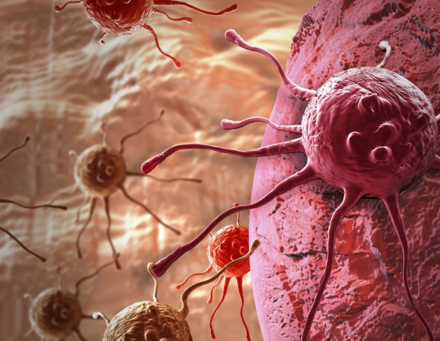
Vitamin B2 metabolism helps cancer cells resist ferroptosis
A lack of vitamin B2 makes tumor cells more susceptible to a unique form of cell death. This was discovered by researchers at the Rudolf Virchow Centre at the University of Würzburg.
The human body cannot produce vitamin B2 –…
Continue Reading
-
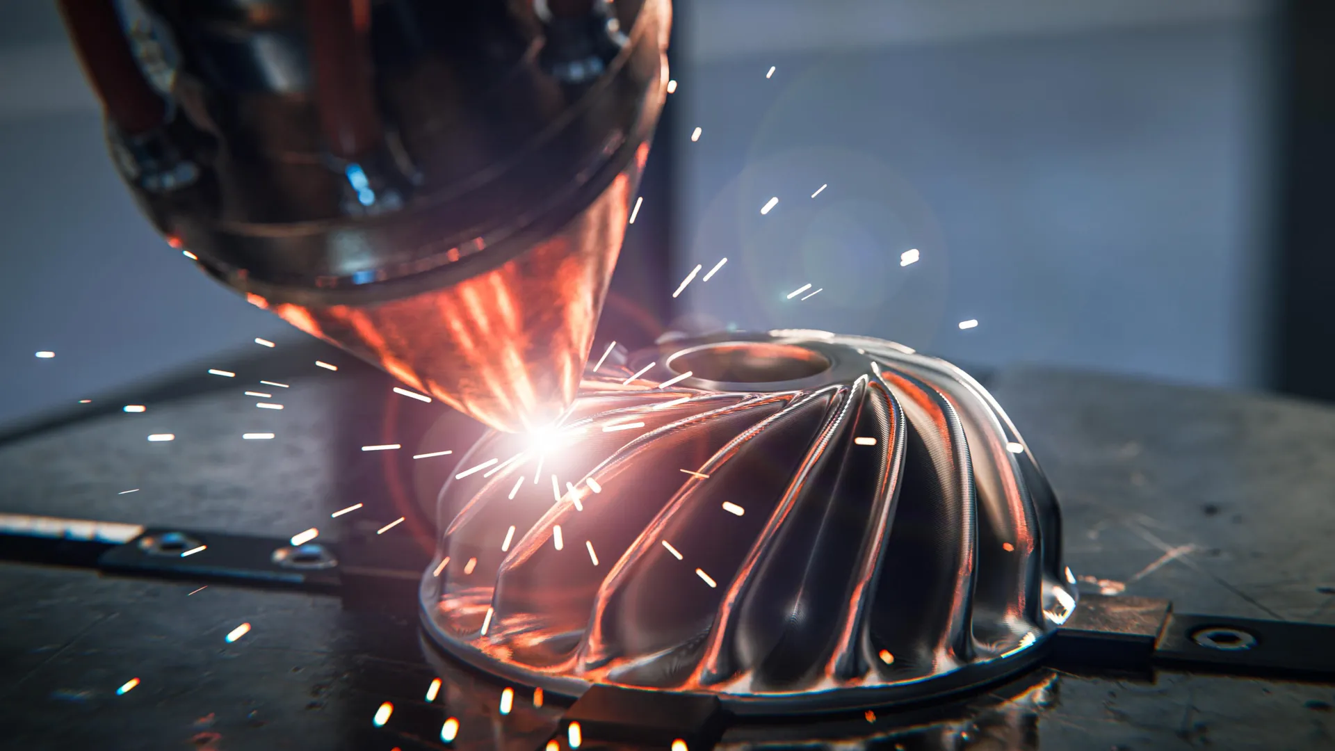
Scientists just found a way to 3D print one of the hardest metals on Earth
Tungsten carbide-cobalt (WC-Co) is widely valued for its extreme hardness, but that same strength also makes it very difficult to shape and manufacture. Current production methods consume large amounts of costly material while delivering…
Continue Reading