- “At First, We Thought Something Was Wrong” – NASA DART Mission Reveals a Cosmic Snowball Fight SciTechDaily
- Moons around asteroids exchange dust and rocks, reveals study Interesting Engineering
- Dimorphos with color enhanced markings to…
Category: 7. Science
-
“At First, We Thought Something Was Wrong” – NASA DART Mission Reveals a Cosmic Snowball Fight – SciTechDaily
-
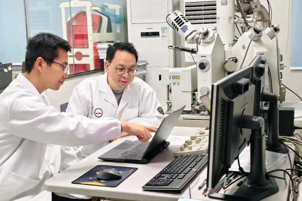
Study on rare earth formation sheds light on future discoveries
Recent research by Chinese scientists explains how deposits of rare earth elements (REE) are formed, proving that the emplacement depth (pressure) of carbonatitic magma is a key factor controlling the abnormal…
Continue Reading
-
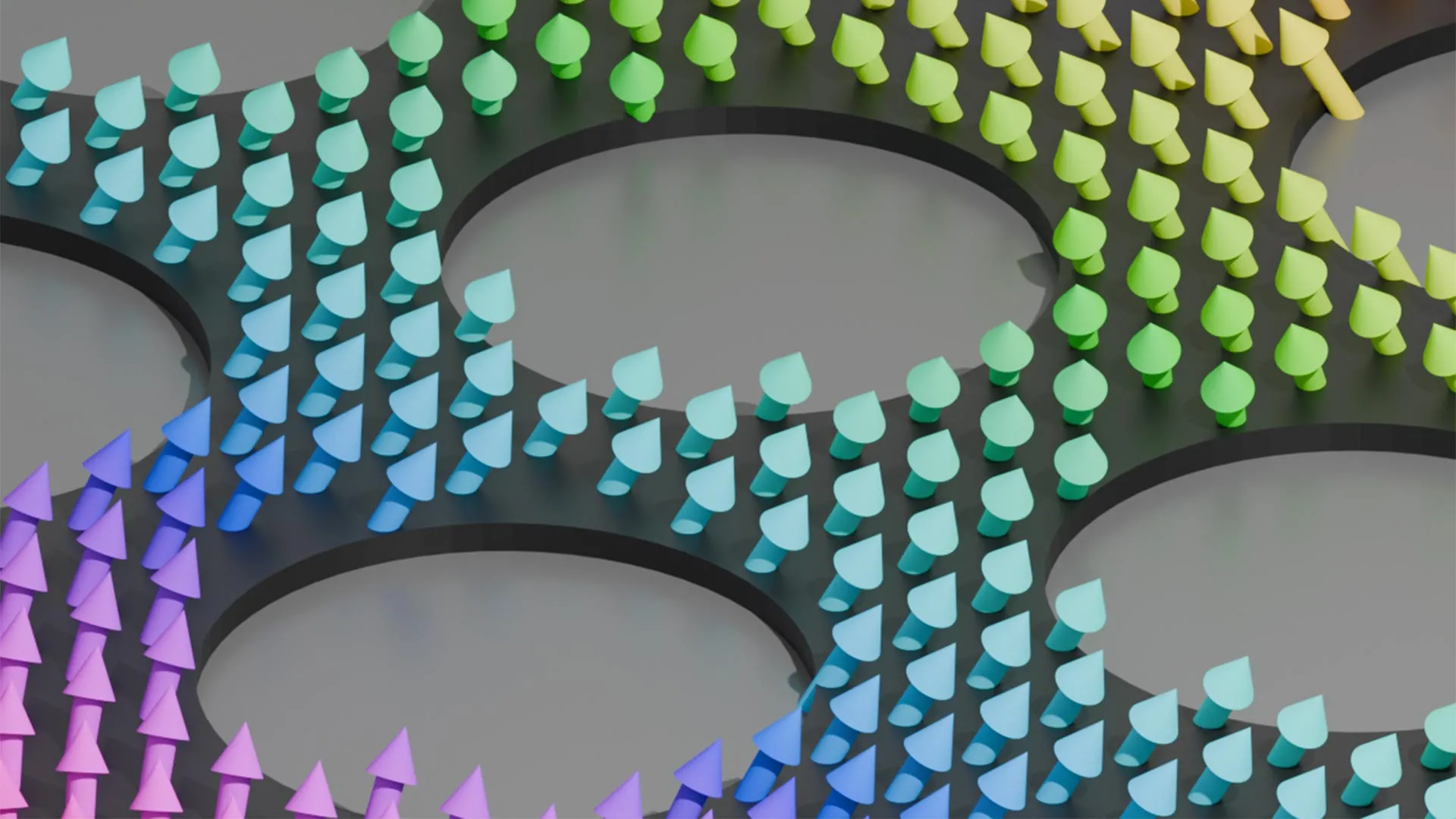
Engineers make magnets behave like graphene
Two dimensional materials have drawn intense interest because their electronic and magnetic properties could power future technologies. Scientists have traditionally treated these two behaviors as separate. Engineers at Illinois Grainger…
Continue Reading
-
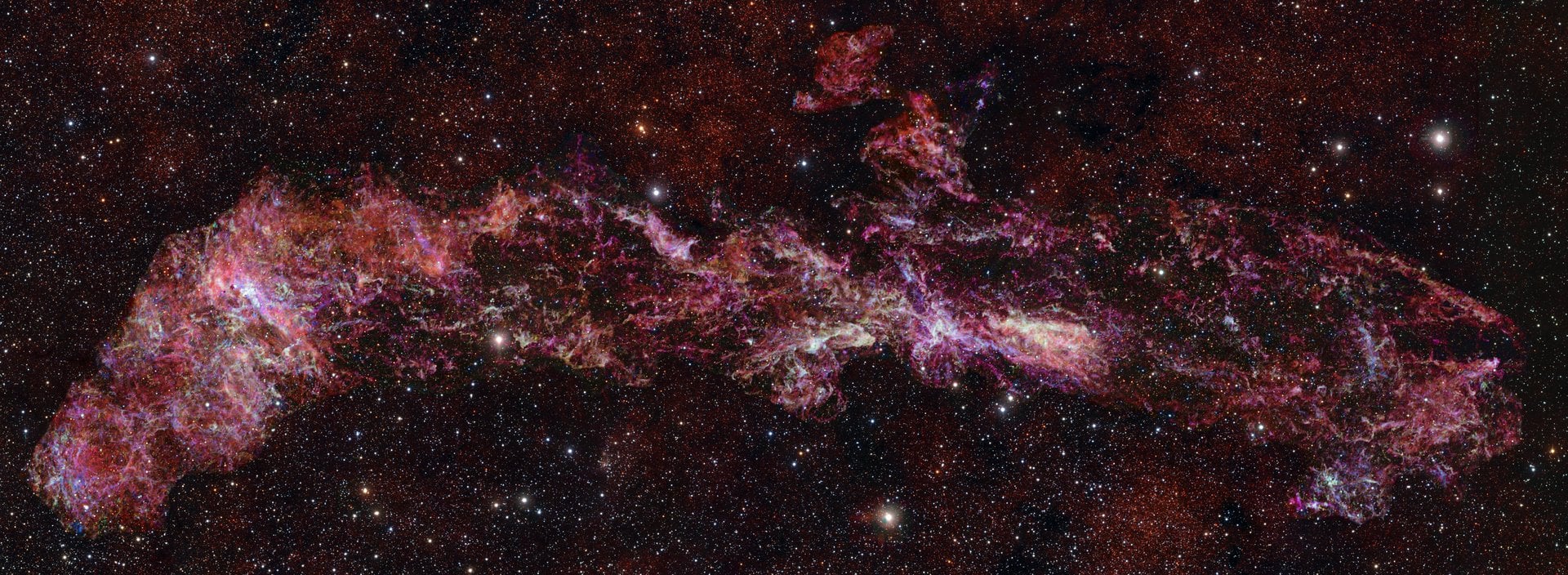
Astronomers Produce the Largest Image Ever Taken of the Heart of the Milky Way
The central region of our Milky Way, sometimes referred to as the “Bulge,” remains something of an enigma to astronomers. Because it is densely packed with stars and clouds of dust and gas, capturing images of its interior has…
Continue Reading
-
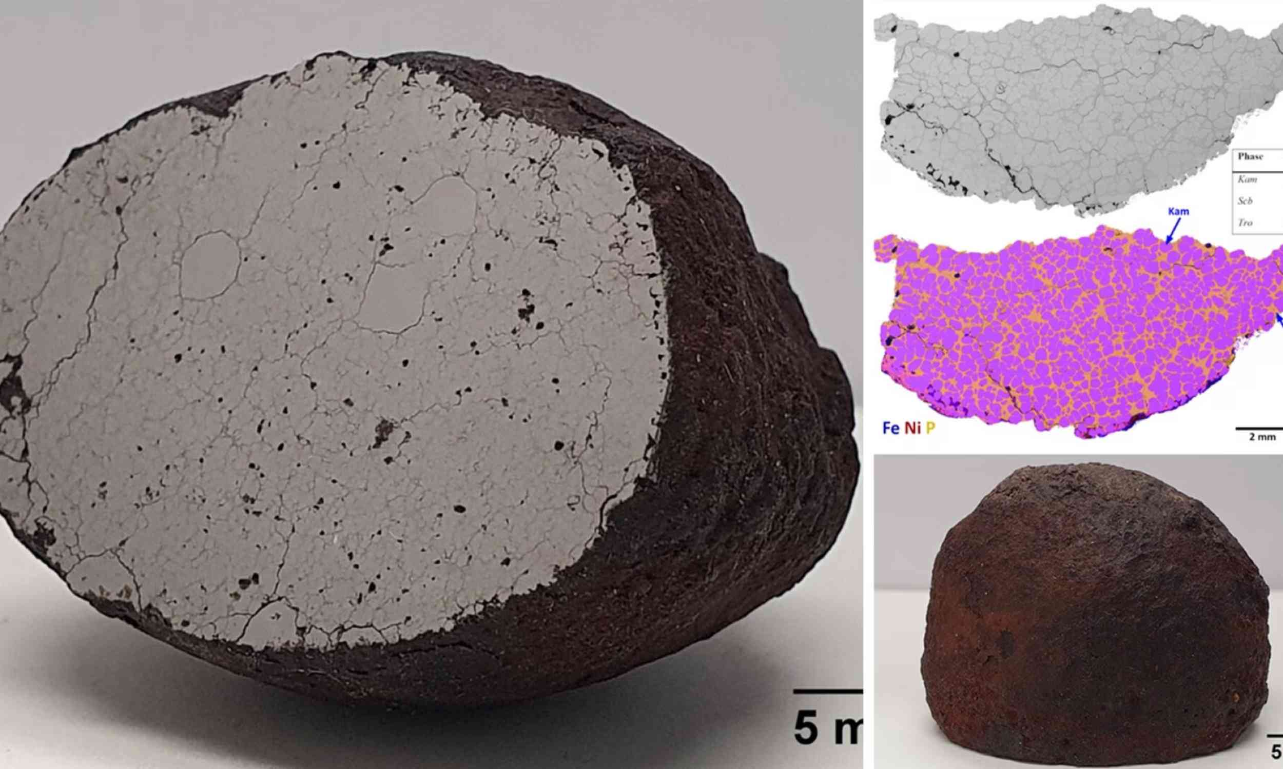
Space rock found in 2017 turns out to be incredibly rare
A small iron meteorite found in Finland has become the most phosphorus-rich iron meteorite ever identified.
Its extreme chemistry preserves a rare record of how metal once separated and reorganized inside a shattered asteroid core.
Inside the cut…
Continue Reading
-

Socially tolerant monkeys have larger emotion centers in the brain
Scientists have discovered that macaque species with more tolerant social systems possess a larger emotion-processing center in the brain.
The finding reframes a brain region long tied to aggression as a core component of how primates manage…
Continue Reading
-
Immunotolerant Oligomer scaffolds promote regenerative remodeling and improved muscle structure and function after volumetric muscle loss
Chi, D. et al. Free functional muscle transfer for lower extremity reconstruction. J. Plast. Reconstr. Aesthet. Surg. 86, 288–299 (2023).
Zhang, Q. et al. Harnessing the synergy of perfusable…
Continue Reading
-
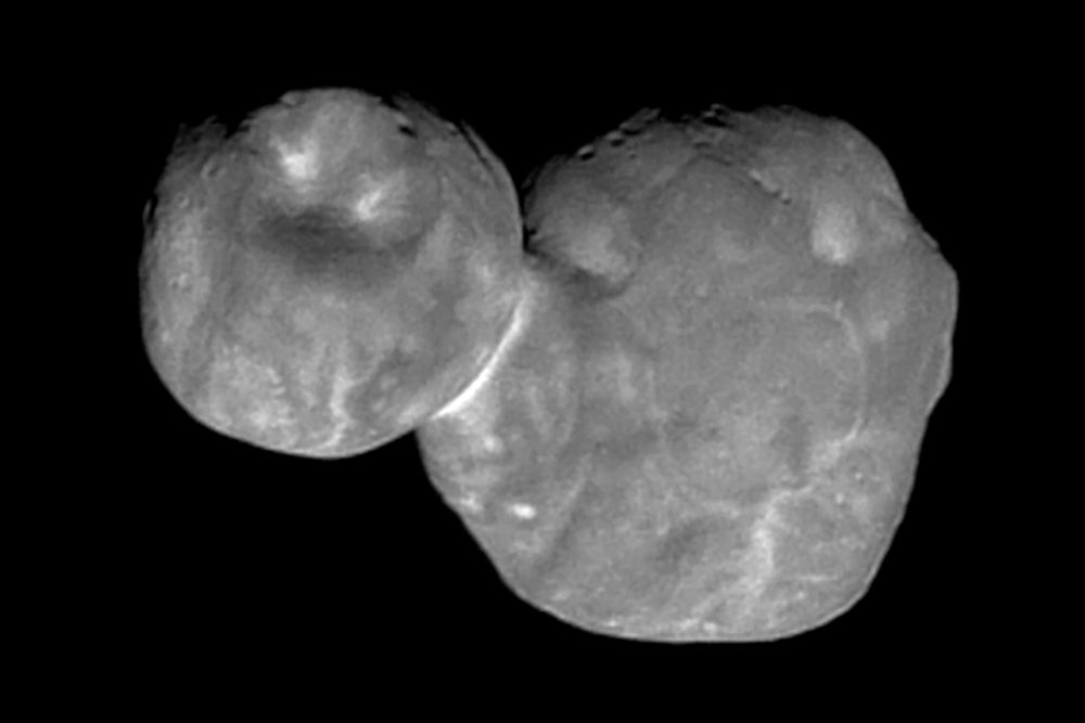
College Student Solves Mystery of ‘Snowmen’ Floating in Space
NEED TO KNOW
-
Graduate student Jackson Barnes appears to have solved how snowman-like objects in space are formed
-
He created a simulation that reproduces the objects known as Arrokoth
-
NASA first spotted the objects with the Hubble Space Telescope in…
Continue Reading
-
-
Scientists stunned to find signs of ancient life in a place no one expected
Dr. Rowan Martindale, a paleoecologist and geobiologist at the University of Texas at Austin, was hiking through the Dadès Valley in Morocco’s Central High Atlas Mountains when something unusual caught her attention and made her stop.
Martindale…
Continue Reading
-

SpaceX springs forward with another Starlink launch from California
Hours after setting clocks forward for Daylight Savings Time, SpaceX went forward with a launch of Starlink satellites on Sunday (March 8).
The Falcon 9 rocket lifted off at 7:00 a.m. EDT (11:00 GMT or 4:00 a.m. PDT local time) from Space Launch…
Continue Reading