Qaasid News
Download Our App
Latest News from Pakistan
CDF Asim Munir tells Afghan Taliban to choose between TTP and Pakistan
December 21, 2025
1,300+ Security Personnel Deployed in Rawalpindi Ahead of PTI Protest
December 21, 2025
Home For The Holidays Flash Sale
December 21, 2025
Transparent nanowire films block 99.97% of electromagnetic noise
December 21, 2025
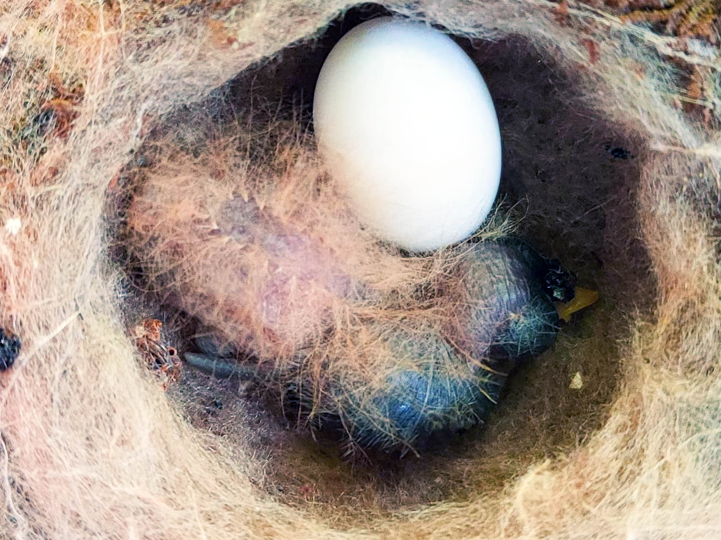
Baby hummingbird seen behaving like a poisonous caterpillar
December 21, 2025
Lightning re-assign forward Jakob Pelletier to AHL Syracuse
December 21, 2025
PM Netanyahu meets with U.S. Senator Lindsey Graham Ministry of Foreign Affairs – www.gov.il
December 21, 2025
Peter Lloyd-Jones obituary | Art and design
December 21, 2025
A Literature Review of the Renal Manifestations in Pediatric Celiac Disease and Its Associated Clinical Implications
December 21, 2025
Level Up Your 2026 With a MasterClass Subscription While It’s 50% Off
December 21, 2025