Qaasid News
Download Our App
Latest News from Pakistan
Italy’s rising star Giovanni Franzoni edges Marco Odermatt to win Kitzbühel downhill
January 24, 2026
Djokovic claims 400th grand slam win to reach Australian Open 4th round-Xinhua
January 24, 2026
A landslide on Indonesia’s Java island kills at least 8 people and leaves more than 80 missing
January 24, 2026
Piers Morgan sends strong message to Donald Trump after Prince Harry’s remarks
January 24, 2026
Iran FM thanks Pakistan for ‘strong support’ at UN Human Rights Council – Dawn
January 24, 2026
Iran FM thanks Pakistan for ‘strong support’ at UN Human Rights Council – Dawn
January 24, 2026
China’s new method boosts productivity by 10x
January 24, 2026
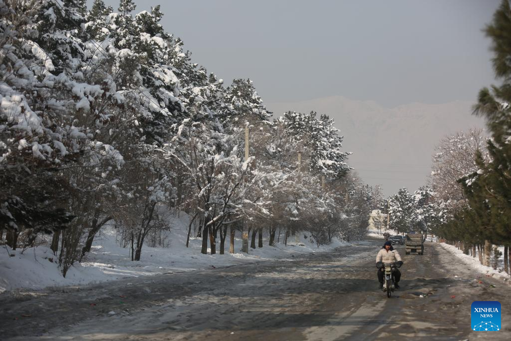
61 killed, 110 injured in heavy snowfall, rains in Afghanistan-Xinhua
January 24, 2026
Milestone man Djokovic reaches Australian Open fourth round
January 24, 2026
Three dead as fire breaks out at Lahore hotel, rescue underway
January 24, 2026