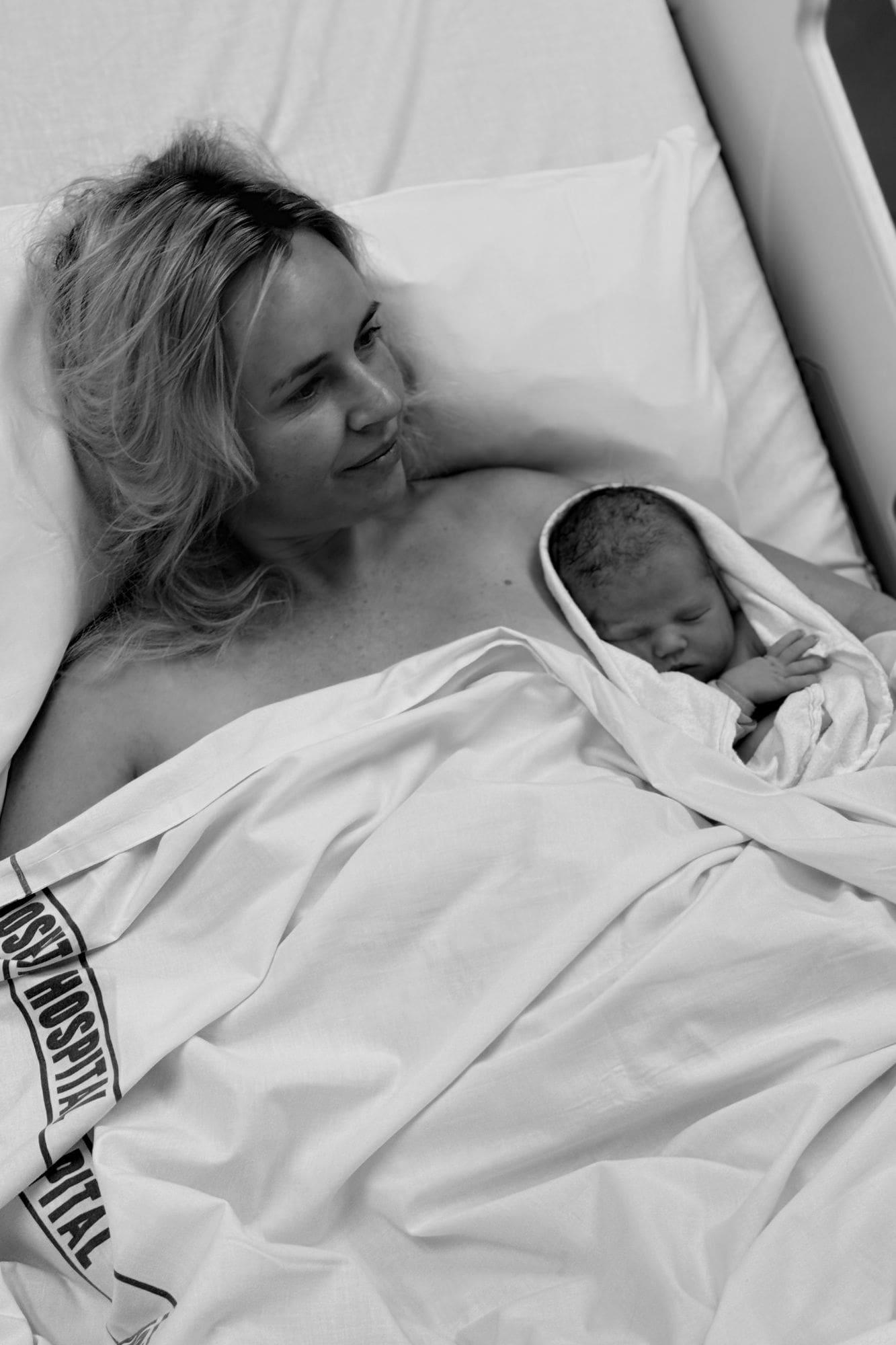
Analysis of the impact of inflammatory and nutritional markers on prognostic factors in lung cancer patients
Univariate analysis
This study ultimately included 500 patients with lung cancer, comprising 178 patients in the survival group and 322 patients in the deceased group. Patients in the survival group had significantly higher levels of lymphocyte count, serum albumin, hemoglobin, prognostic nutritional index (PNI), lymphocyte-to-monocyte ratio (LMR), hemoglobin-to-red cell distribution width ratio (HRR), hemoglobin-albumin-lymphocyte-platelet (HALP) score, albumin-to-globulin ratio (ALB/GLB), as well as a greater proportion of stage I cases and patients with high-to-moderate tumor differentiation. In contrast, patients in the deceased group exhibited significantly higher levels of serum globulin, age, systemic immune-inflammation index (SII Log), platelet-to-lymphocyte ratio (PLR Log), neutrophil-to-lymphocyte ratio (NLR), and a higher proportion of cases with distant metastasis, stage IV disease, Eastern Cooperative Oncology Group performance status (ECOG PS) ≥ 2, and poorly differentiated tumors. Table 1.
LASSO regression analysis and risk prediction formula
In this study, mortality in lung cancer patients was used as the dependent variable. Independent variables included clinical stage (coded as 1 = Stage I, 0 = Stage II/III/IV), differentiation grade (coded as 1 = low differentiation, 0 = moderate/high differentiation), ECOG PS (coded as 1 = ECOG PS 0–1, 0 = ECOG PS ≥ 2), serum albumin (measured value), LMR (measured value), HRR (measured value), ALB/GLB (measured value), and age (measured value).LASSO regression analysis identified ECOG PS 0–1, ALB/GLB, and age as independent prognostic factors for lung cancer. ECOG PS 0–1 and higher ALB/GLB levels were protective factors, while age was a significant risk factor. Specifically, the analysis indicated that each additional year of age increased the risk of mortality by approximately 7%.Table 2. The following formula was provided to calculate the mortality risk prediction score for individual patients: Exp(x) = [−0.94909] + [−0.47464 × 1(Stage I)] + [0.54761 × 1(Low differentiation)] + [−0.85073 × 1(ECOG PS 0–1)] + [−0.00427 × Serum albumin] + [−0.04974 × LMR] + [−0.28638 × HRR] + [−0.98366 × ALB/GLB] + [0.06838 × Age].The probability of mortality is calculated as: Probability = Exp(x)/[1 + Exp(x)].
Development of a risk prediction model
Feature selection using LASSO regression for dimensionality reduction
In this study, LASSO regression analysis with 10-fold cross-validation was used to select the optimal log(λ) values. When log(λ) was − 2.8203 and − 3.5645, the data demonstrated stability and statistical significance. Figure 2 shows the coefficient distribution curve for different log(λ) values. Figure 3 illustrates the stepwise feature selection process, reducing 46 variables to 1. Each curve represents the trajectory of different predictor coefficients as the parameter changes.The optimal eight variables selected for constructing the lung cancer risk prediction model based on inflammation and nutrition markers were: age, Stage I, low differentiation, ECOG PS 0–1, serum albumin, LMR, HRR, and ALB/GLB.Age was identified as an independent risk factor for poor prognosis, with increasing age associated with worse outcomes. Patients with Stage I disease and ECOG PS 0–1 had better prognoses. In contrast, low differentiation, decreased serum albumin levels, and lower ALB/GLB were associated with worse outcomes. Elevated LMR and HRR were linked to improved prognosis.Table 3. Figure 2. Figure 3.
Cross-validation of LASSO regression analysis. Note: The vertical axis represents the cross-validation error, which serves as a metric for assessing model goodness-of-fit. A smaller value indicates better model fit. The lower horizontal axis corresponds to log(λ), where λ is the regularization parameter that controls the complexity of the model. The upper horizontal axis denotes the number of variables retained at different log(λ) values. The two vertical dashed lines indicate the optimal log(λ) value and the log(λ) value within one standard error. Specifically, the upper horizontal axis value corresponding to the left dashed line represents the number of selected variables at the optimal log(λ) value.

Variable selection path in LASSO regression. Each line in a different color represents a variable. The bottom x-axis corresponds to log(λ) values, while the top x-axis indicates the number of nonzero coefficients (variables) in the model for the respective log(λ) values. The log(λ) value controls the strength of regularization in the model: smaller log(λ) values correspond to weaker regularization, allowing more variables to enter the model, whereas larger log(λ) values correspond to stronger regularization, enhancing the model’s robustness to noise but shrinking many variable coefficients to zero.As the log(λ) value increases (from smaller to larger values), the model complexity decreases, with many variable coefficients gradually shrinking to zero or becoming exactly zero. However, the coefficients of certain variables remain nonzero throughout the process. This observation suggests that the model identifies these variables as more critical features, enabling dimensionality reduction or the selection of the most important predictors.
Near-Zero variance test of training data
To further refine variable selection and understand their local characteristics and distribution patterns, a near-zero variance test was conducted on multiple variables. The results showed that patient age, ALB/GLB, and ECOG PS scores (≥ 2 and 0–1) were evenly distributed, suggesting their relevance to prognosis. The proportions of LMR, HRR, and ALB/GLB were 93.79%, 94.99%, and 98.20%, respectively, indicating high individual variability among these variables.Table 4.
Collinearity test on training data (Stepwise VIF Selection)
To improve the predictive performance of the model and address irrelevant variables, a collinearity test (VIF) was performed to further refine the feature selection. Variables such as Stage II, moderate/high differentiation, and ECOG PS ≥ 2 were stepwise excluded. The retained variables included Stage I, Stage III, Stage IV, low differentiation, ECOG PS 0–1, serum albumin (g/L), LMR, HRR, ALB/GLB, and age.The analysis identified age, clinical stage, low differentiation, ECOG PS 0–1, serum albumin levels, LMR, HRR, and ALB/GLB as independent prognostic factors.Table 5.
Recursive feature elimination
To identify the most relevant feature variables, recursive feature elimination (RFE) was performed. The selected variables included Stage I, low differentiation, ECOG PS 0–1, serum albumin (g/L), LMR, HRR, ALB/GLB, and age.The analysis revealed that LMR had the most significant predictive performance. Serum albumin, ALB/GLB, and HRR also demonstrated strong predictive capabilities. Age, Stage I, low differentiation, and ECOG PS 0–1 showed moderate predictive value.Table 6.
Variable importance
Finally, this study systematically evaluated the factors influencing prognosis and identified age as the most critical determinant. The factors ranked in descending order of impact were ECOG PS 0–1, ALB/GLB, poor differentiation, stage I, HRR, LMR, and serum albumin. Table 7.
Model evaluation
ROC curve (Internal validation performed 500 Times)
The performance of the model was evaluated using the ROC curve, with an area under the curve (AUC) of 0.7652 (95% CI: 0.7246–0.8029) and an accuracy of 0.711 (95% CI: 0.669–0.751). The model demonstrated high sensitivity (0.847) and moderate specificity (0.466), indicating good discriminatory power, making it suitable for preliminary disease screening. The positive predictive value (0.741) exceeded the negative predictive value (0.629), suggesting the model is more reliable in identifying positive cases.Internal validation was conducted using 500 bootstrap resamples. Calibration was assessed with isotonic regression fitting. The results showed an F1-score of 0.791 (range: 0–1, with higher values indicating better balance), confirming that the model achieved a good trade-off between precision and recall. These findings highlight the model’s strong predictive accuracy, good sensitivity, and reliable calibration, demonstrating its overall predictive and fitting performance.Table 8. Figure 4.

Optimal cutoff point
The ROC cut-off points, sensitivity, and specificity for eight inflammation-nutritional markers, including NLR, PLR, SII, LMR, PNI, HALP, HRR, and ALB/GLB, are presented in Supplementary Table S1. Users can select appropriate cut-off points based on their clinical context to predict future outcomes (see Supplementary_Table_S1.pdf).
Model calibration
The predictive performance of the model was evaluated using a visual calibration curve. The calibration curve closely aligned with the ideal curve, with a slope of 1. This indicates that the risk prediction model has good calibration performance and can provide reliable risk estimates. Figure 5.

Calibration plot for the predictive model in the training dataset.
Clinical utility of the model
The decision curve analysis demonstrated that the predictive model (PRED.MODEL1) maintained stable performance across various risk thresholds. In the low-risk range (0.2–0.3), the model effectively identified high-risk patients requiring intervention while reducing overtreatment. In the moderate-risk range (0.3–0.6), it performed optimally, balancing treatment benefits with potential risks. Even in the high-risk range (0.6–0.8), the model retained good discriminatory ability, aiding in the identification of patients needing aggressive intervention.The model’s curve consistently remained above the reference line and was most prominent in the moderate-risk range (0.3–0.6). These findings indicate that the predictive model can effectively guide clinical decision-making. Figure 6.

Decision curve analysis of PRED.MODEL1 for clinical decision-making.
Web-Based calculator for prognostic risk prediction in patients with lung cancer
We have developed a web-based calculator for predicting the prognostic risk of lung cancer patients. Instructions for Use: After accessing Risk Prediction Model for Overall Survival in Lung Cancer Patients, input the patient’s information as follows: Select “Yes” or “No” for “Stage I.“Select “Yes” or “No” for “Poor Differentiation.“Select “Yes” or “No” for “ECOG PS 0–1.“Enter the serum albumin level (g/L) in the designated field.Input the LMR, HRR, and ALB/GLB values in their respective fields.Enter the patient’s age in years.Once all fields are completed, click “Calculate Risk.” The probability of mortality for lung cancer patients will be automatically displayed at the bottom of the interface. For reference, see the webpage calculator interface in Fig. 7.

Shows the interface of the web-based calculator.