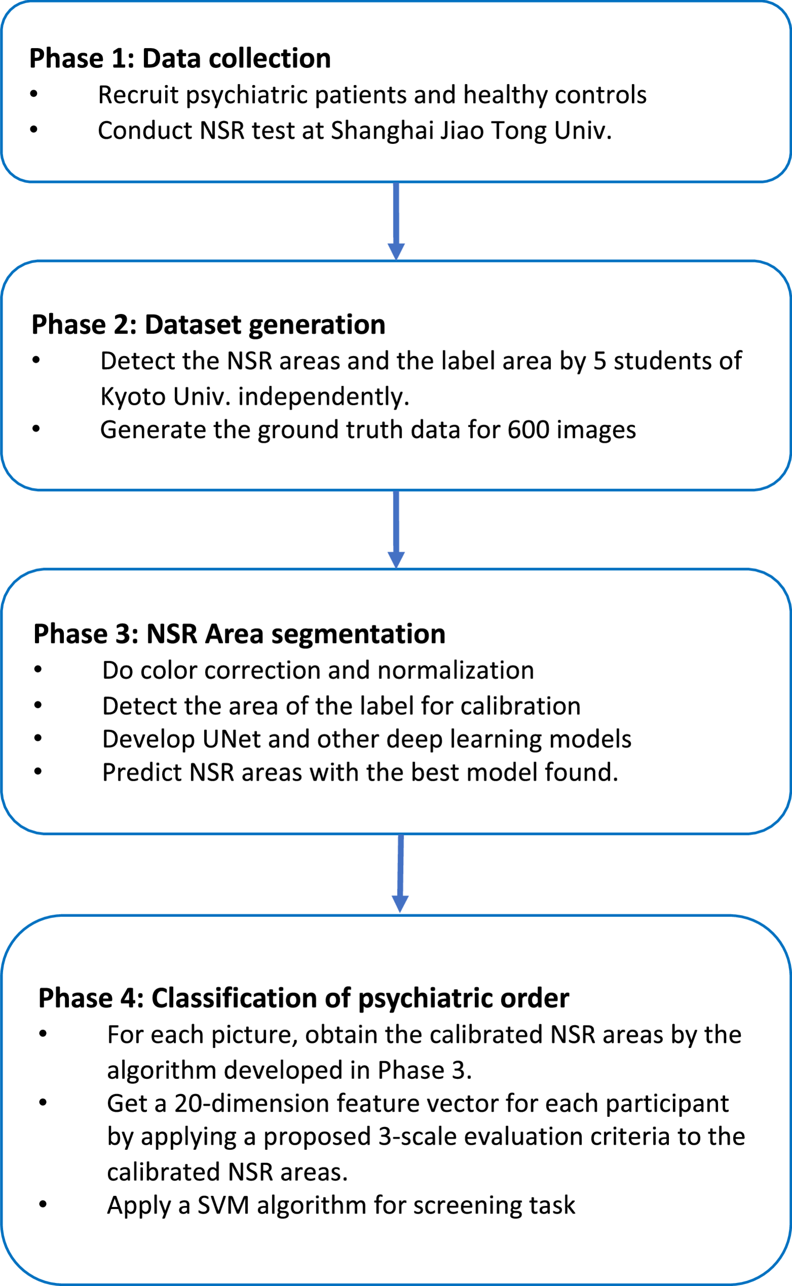
The data analysis pipeline was bifurcated into two primary stages: precise NSR area detection via Deep Learning-based segmentation, followed by Machine Learning (ML) classification for psychiatric disorder screening.
Image pre-processing and data augmentation
To prepare the raw NSR images for analysis and enhance model performance, a series of pre-processing and augmentation steps were applied. Initially, color correction was performed using the Perfect Reflector Method, leveraging the white section of the included label as a standardized white reference to mitigate color inconsistencies arising from diverse acquisition devices and varying lighting conditions. Concurrently, an image size normalization step was executed by utilizing the consistent real-life size of the arm label as a reference, thereby compensating for variations in camera-to-arm distances across different tests. After these initial corrections, all images were uniformly resized to 512 × 128 pixels, a rectangular aspect ratio optimized for the input requirements of the subsequent Deep Learning models.
To significantly bolster the robustness and generalization capabilities of our segmentation models, runtime data augmentation was extensively implemented during the training phase using the Albumentations library (https://albumentations.ai/). This dynamic augmentation strategy involved applying various transformations such as random rotations, shifts, scaling, flips (horizontal/vertical), and controlled adjustments to brightness, contrast, and saturation. This approach allowed the models to learn more invariant and discriminative features, reducing overfitting and improving performance on unseen data.
NSR area detection (segmentation)
For the critical task of identifying and segmenting the subtle NSR areas, which often exhibit low contrast and indistinct boundaries, an advanced Deep Learning approach was adopted. This project explored multiple state-of-the-art segmentation models to identify the most effective architecture for the task. We chose the following Deep Learning models Vit-Unet, Resnet152-Unet, Effb5-Unet, Mob-Deeplab, Mob-DeeplabPlus, Resnet152-Unet++, and plain UNet because they are encoder-decoder based semantic segmentation models known for efficiency and robust performance in medical image analysis, particularly with limited computational resources and data. Their proven capabilities in producing dense pixel-wise predictions, their relative computational efficiency for training on a new dataset, and their interpretability in identifying precise regions made them suitable for our initial objective of establishing a robust and efficient baseline.
We remark that while Mask R-CNN and DeepLabV3 + are prominent architectures in the field of computer vision, they were not the primary focus for this particular segmentation task for a few key reasons. Mask R-CNN, primarily an instance segmentation model, is optimized for detecting and segmenting individual objects within an image. Our task, however, is a semantic segmentation problem, where we are interested in identifying a single, continuous region (the flushed area) rather than individual instances. Applying Mask R-CNN directly would be an overkill and potentially less efficient for this specific problem type, possibly leading to unnecessary computational overhead and complexity in post-processing to consolidate instances into a single semantic region. DeepLabV3+, on the other hand, is a powerful semantic segmentation model but often leverages dilated convolutions and large receptive fields, which can be computationally intensive and might require larger datasets or more aggressive training strategies to generalize effectively on fine-grained segmentation tasks like NSR, especially given the subtle boundaries. Our objective is to establish a robust and efficient baseline, making encoder-decoder architectures, particularly U-Net variants known for their efficacy in biomedical image segmentation, more suitable for a direct comparative evaluation on our curated dataset.
Among the evaluated models, the Efficient-Unet (Effb5-Unet) architecture consistently demonstrated superior performance in accurately segmenting the NSR areas from the corrected and augmented images. The comprehensive dataset was divided into distinct sets for training, validation, and testing at the patient level, ensuring that no patient’s data appeared in more than one set. Since there are 120 unique participants, this rigorous partitioning involved 90 of them for training, 10 for validation, and 20 for independent testing. Models were trained using standard optimization protocols, with performance monitored via common metrics including Dice coefficient and Intersection over Union (IoU). We employed no post-processing since the results were good enough and we wanted to directly compare the Deep Learning models only.
NSR quantification and screening approaches
Following the NSR area detection, we explored various methods to quantify the NSR and subsequently screen for psychiatric disorders. Previous studies have utilized a 4-point scale for measuring NSR degrees. Recognizing the inherent subjectivity of manual annotation, we developed a more objective 3-scale, derived from the automatically detected NSR areas and their correspondence to manually assigned scores (see the following). Besides this score-based approach, we also applied a direct screening method utilizing the raw detected NSR areas, bypassing discrete score assignment. A comparative analysis of these methods was performed to corroborate the efficacy of our proposed objective quantification.
NSR area scoring (objective 3-scale)
For each detected region, we calculate the normalized area, Anorm, as the ratio of the detected NSR area Adetected to the corresponding labeled area Alabel (the area of the label attached to the arm), i.e.,
Anorm = Adetected/ Alabel.
We then analyzed the mean value, variance, and standard deviation of the normalized area distributions corresponding to each human score. The observed results were as follows: For score 0, the mean value, variance, and the standard deviation were 0.0648, 0.0229, and 0.1515, respectively. For score 1, they were 0.1535, 0.0363, and 0.1907, respectively. For score 2, they were 0.1661, 0.0217, and 0.1477, respectively. And for score 3, they were 0.1665, 0.0291, and 0.1706, respectively. While the distributions of the normalized areas vary across different scores, there is a considerable overlap and variance. Consequently, we established the next objective 3-scale scoring system based on the above observations:
Score 0 if Anorm < 0.1091; Score 1 if 0.1091 ≤ Anorm < 0.1598; and Score 2 otherwise.
Feature extraction for classfication
For each participant, based on the NSR areas detected by the Efficient-Unet model, we created two distinct types of 20-dimensional feature vectors for classification, each capturing the scores of normalized sizes of the four NSR areas at five critical time points (1st, 5th, 10th, 15th, and 20th minute) post-application. Firstly, we established the objective 3-scale score-based feature vector as explained before. Each element represented the objectively derived 3-scale score (0, 1, or 2) for a specific niacin patch concentration at a given time point. Secondly, we established the direct NSR area feature vector. Each element represented the normalized NSR area Anorm directly for a specific niacin patch concentration at a given time point. This vector comprehensively captured the dynamic and concentration-dependent physiological response with high granularity and objectivity, without discrete score assignment.
Psychiatric disorder screening (classification)
The final stage of the analysis involved classifying participants into specific diagnostic groups based on their extracted NSR feature vectors. A Support Vector Machine (SVM), a robust supervised learning model well-suited for high-dimensional data, was selected for this classification task. To ensure the SVM’s performance was optimized and robust against potential biases, several advanced techniques were employed.
5-Fold cross-validation
The entire dataset of feature vectors was subjected to 5-fold cross-validation. In each iteration, 80% of the data served as the training set, and the remaining 20% as the test set, ensuring a comprehensive and reliable evaluation of the model’s generalization capabilities. This process was iteratively performed until each subset had been used as the test set once.
SMOTE for class imbalance
Given the inherent class imbalances often present in clinical datasets, the Synthetic Minority Over-sampling Technique (SMOTE) was applied to the training data within each cross-validation fold. This algorithm synthesized new minority class samples, thereby balancing the class distribution and preventing the SVM from being unduly biased towards the majority healthy control group.
Hyperparameter tuning
Extensive grid search was performed within each cross-validation fold to ascertain the optimal hyperparameters for the SVM model (e.g., kernel function (radial basis function was generally preferred), ‘C’ regularization parameter, and ‘gamma’ for RBF kernel). This meticulous tuning aimed to maximize the balanced accuracy of the classifier, a crucial metric for imbalanced datasets, thereby pushing the SVM’s predictive performance to its empirical limit.
The final classification performance was evaluated using standard metrics including overall accuracy, as well as class-specific precision, recall (sensitivity), and specificity, across various binary classification tasks (e.g., HC vs. Depression, HC vs. Schizophrenia, HC vs. Bipolar Disorder).