
TAMPA, Fla. – January 9, 2026 – The…
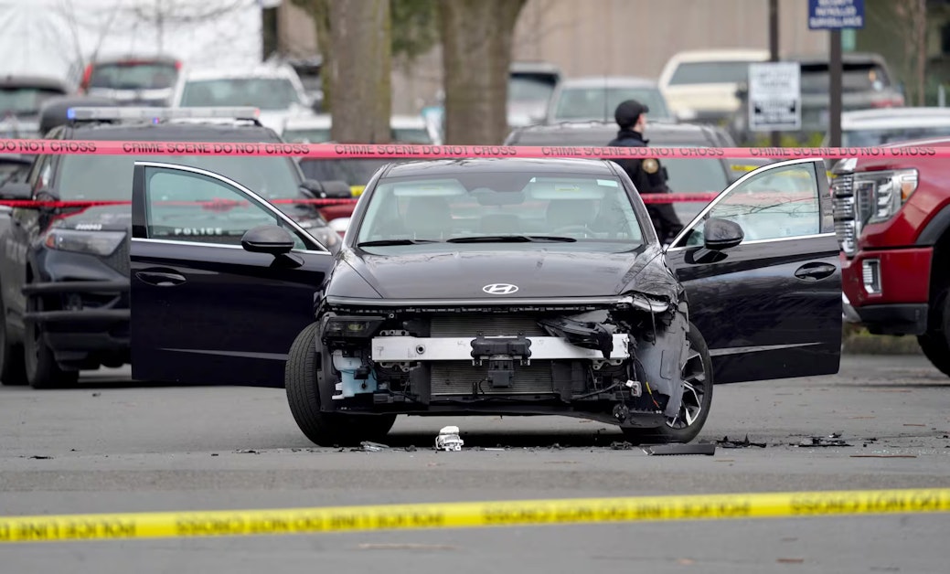
Update, 7:20 am. on Friday, 1/9/26: The U.S. Department of Homeland Security has identified the people shot in Portland yesterday as Luis David Nico Moncada and Yorlenys Betzabeth Zambrano-Contreras, both from Venezuela. DHS…