CAIRO, Nov. 18 (Xinhua) — Egyptian President Abdel-Fattah al-Sisi and British Prime Minister Keir Starmer held a phone conversation on Tuesday, during which they emphasized the urgent need to build upon the recent UN Security Council…
The European Molecular Biology Laboratory’s European Bioinformatics Institute (EMBL-EBI) today announced the launch of a new online hub for global antimicrobial resistance (AMR) data.
Launched with the aim of making global AMR data more accessible…
Eminem has taken legal action against Sydney-based beach company Swim Shady, alleging the brand’s name infringes on his trademarked rap alter ego Slim Shady, the BBC reports.
The Rock and Roll Hall of Famer’s attorneys contend that the beach…
The 19th-century building (which was originally built for dried good storage) was later the home of abstract expressionist Barnett Newman. “He had this floor and the one below us because apparently he didn’t want to hear anyone walking around…
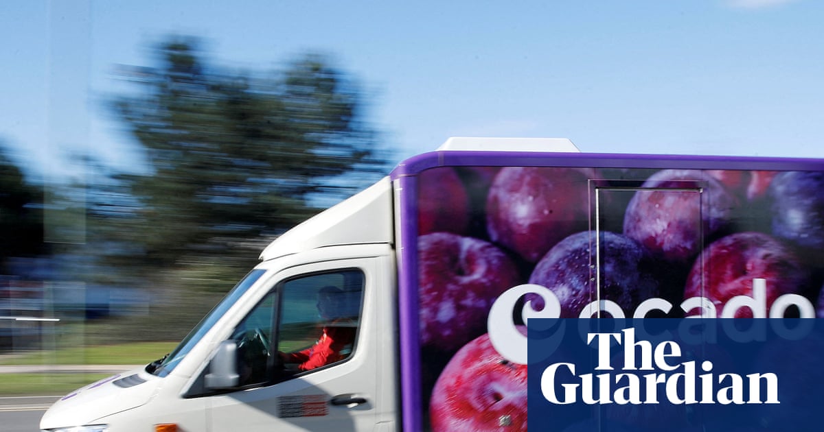
The value of online grocer Ocado has fallen sharply after Kroger, it’s major partner in the US, announced the closure of three warehouses using the UK company’s high-tech equipment.
Ocado signed a deal to build 20 automated warehouses – known as customer fulfilment centres – for Kroger, the US’s fourth largest retailer, in 2018. Eight of those facilities are currently operating with two more planned for next year. The deal was seen as a major part of Ocado’s plan to sell its online grocery delivery technology internationally.
However, on Tuesday, Kroger said sites in Frederick in Maryland, Pleasant Prairie in Wisconsin, and Groveland in Florida would close in January. Shares in Ocado were down more than 17% on Tuesday after the announcement, wiping about £350m off the value of the company.
Kroger said that after reviewing its set-up it had “identified opportunities to optimise its fulfilment network”.
It added that it would now move towards a “hybrid fulfilment network” testing out “capital-light, store-based automation in high-volume geographies” while continuing to use automated warehouse processing of online orders where it sees “higher density of demand”. It noted that it had recently expanded its relationship with quick delivery service providers DoorDash, Instacart and Uber Eats, which take goods directly from stores on bikes, mopeds and other small vehicles.
Clive Black, a retail analyst at Shore Capital, described Kroger’s announcement as a “near knockout punch” for Ocado, prompting the share price to fall below the 180p price at which it debuted on the London stock market in 2018.
He said the online grocery technology supplier “is being marginalised as most of its customer fulfilment centres do not work economically in the USA or the mass-market first world in truth.”.
While centralised, automated warehouses may work effectively to manage home deliveries of groceries in densely populated and affluent urban locations, according to Black, he said Kroger’s actions suggested that the size of Ocado’s total potential market “has been blitzed”.
“We had expected Kroger to trundle on, not close [warehouses], as part of its ongoing review, a dreadful acclamation of what Morrison, Waitrose and others already knew: capital intensive, centralised fulfilment of food to a dispersed mass-market customer does not financially work.”
Ocado said it expected to receive more than $250m (£190m) in compensation for fees related to the early closure of the sites but its fee revenue would take a $50m hit in the financial year to December 2026.
skip past newsletter promotion
after newsletter promotion
“Ocado continues to support Kroger to optimise logistics operations and drive profitable volume growth in these remaining sites, with constructive ongoing discussions around further use of Ocado’s technology to support Kroger,” the British company said in a statement.
It added that it “expects significant growth in the US market, both with [warehousing] and store based automation.”
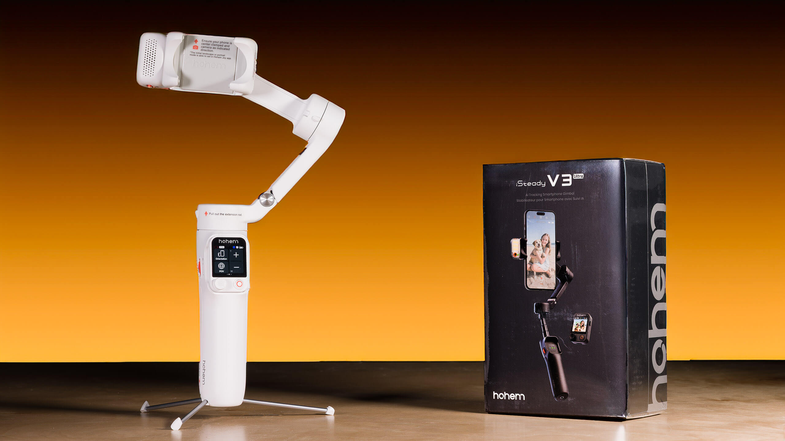
This gimbal is full-featured thanks to the included AI tracking module that doubles as a fill light. The motors stand up to even the heaviest iPhone 17 Pro Max, providing smooth movements. It is lightweight and folds into a compact, easy-to-carry…
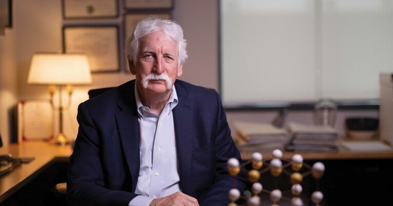
Like many successful researchers, Jorgensen has been guided by scientific pursuits his entire life.
As a kid growing up in Port Washington, a hamlet on the western side of Long Island, and later in Sherman, Connecticut, he conducted scores of experiments with his trusty A.C. Gilbert chemistry set, tromping off to the local drug store regularly to replenish his supply of potassium nitrate. In high school, at Phillips Exeter Academy in New Hampshire, he took AP Chemistry and taught himself how to write computer code in BASIC.
He went on to graduate from Princeton in three years, learning the computer language FORTRAN in the basement of the Frick Lab and conducting work for his first co-authored study in the Journal of the American Chemical Society. Then it was on to Harvard for graduate school (where he worked with eventual Nobel winner EJ Corey), and to Purdue to begin his teaching and independent research career.
He soon came to focus his research on the need for better simulations of systems in solution.
“I realized very quickly that I wanted to study reactions in liquids and investigate the way molecules recognize each other in solution, which can lead eventually to drug design,” Jorgensen said. “In drug design you typically have an inhibitor, a small molecule that is binding to a disease-causing protein, which then disrupts the function of that protein.”
To do this work, he needed computing know-how and processing muscle. So, he taught himself statistical mechanics to go with his working knowledge of programming, and he got together funding for a research computer.
In the late 1970s, Purdue had two CDC 6400s (an early mainframe computer built by the Control Data Corporation) in its computer center. That meant two processors for 40,000 students and faculty, compared to today when the average laptop computer has eight processors. But times were changing.
“Fortunately, I was in the right place at the right time, because by the early 1980s computer resources became more available,” Jorgensen said. “You could have your own computer in your lab, if you could find the money to buy it.”
He and his research group purchased a Harris 80 — a tall cabinet computer that occupied its own room with an air conditioner and a printer. Much of the funding for it came from a 1978 grant to Jorgensen from the National Science Foundation (NSF).
“NSF was essential to the early work I did, including the water models,” Jorgensen said. “NSF funded basic science research that led to many of the technologies and therapeutics we take for granted today.”
Meanwhile, the older guard of scientists, who’d previously held computer modeling at arm’s length began to see the value of adapting to changing technology. “In the late 1970s you had people still trying to do paper-and-pencil theory work, but you also had the new people coming in with their computers,” Jorgensen said. “There was some difficulty in my being accepted by some of the theoretical chemists at the time, who were rather dismissive of what I was doing. I had to prove I could do something useful.”
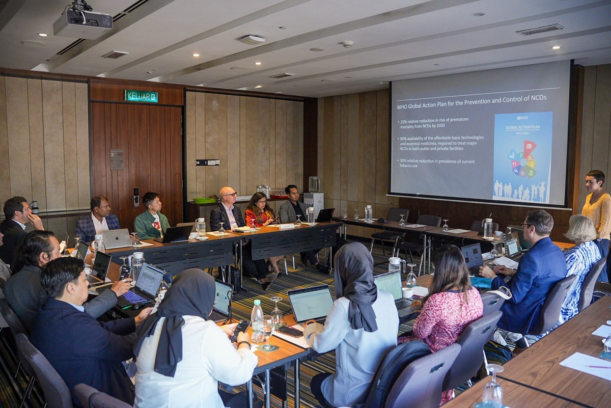
Chronic obstructive pulmonary disease (COPD) is the third leading cause of death globally, yet the condition is relatively unknown and often underprioritized and underfunded. This is despite the fact that over 3.5 million people die from COPD…
More than 80 countries have joined a call for a roadmap to phasing out fossil fuels, in a dramatic intervention into stuck negotiations at the UN Cop30 climate summit.
Countries from Africa, Asia, Latin America and the Pacific joined with EU…