Based on multibody dynamics (ADAMS2020, https://hexagon.com/products/product-groups/computer-aided-engineering-software/adams) integrated with full-well drill string dynamics theory, comprehensive drill string assembly modeling, rate of penetration (ROP) model, and reamer force analysis model from the top drive to the bit were established.
Drill string assembly model
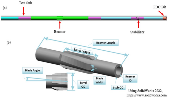
A well in Dagang Oilfield was selected as the case study, with the drill string assembly configuration: PDC bit + double box sub + Stabilizer + float valve with crossover sub + crossover sub + reamer + testing sub + 42 sections of heavy-weight drill pipe + 372 sections of drill pipe. The distance between the bit and the reamer is 6.9 m, and the bit depth is approximately 3993 m. The established reamer model primarily considers its tool body length, OD and ID, as well as the length, orientation angle, and outer diameter of the blades. Figure 1 shows the reamer geometric model and the BHA model.
Rate of penetration model
Since rock-breaking simulation is not included in the dynamic simulation, the ROP (rate of penetration) must be modeled using a nonlinear spring-damping function. During the hypothetical rock-breaking process, an axial load acts between the wellbore wall and the reamer, while the wellbore wall interacts with the formation via spring and damping forces. Based on Newton’s second law, the bottomhole dynamic equation is formulated as Eq. (1), the ROP response is shown in Fig. 2, where Fig. 2(a) represents the theoretical calculation of ROP and Fig. 2(b) depicts the software simulation response of ROP:
$$mS^{primeprime}+cS^{prime}+kS=Kleft( {ROPcdot t+{c_R}} right)+ccdot ROP+{F_b}left[ {a+vcdot sin (omega t)} right]+mg$$
(1)
where m is the mass of the wellbore wall (kg); c is the damping coefficient of the wellbore wall (N/(m/s)), change with well depth; k is the spring stiffness coefficient of the wellbore wall (N/m), change with well depth; g is gravitational acceleration (m/s²); ROP is the mechanical rate of penetration at the bit (m/s); CR is the initial condition for the differential equation governing the ROP input parameter at the bit; Fb is the amplitude of the sinusoidal WOB fluctuation load (kN); a is the constant coefficient term in the sinusoidal WOB fluctuation load.
Weight on bit model
The WOB model is constructed using the STEP, VARVAL, and DIF functions in Adams, Eq. (2)~3: the input WOB is introduced into the hookload function via the STEP function, where the hookload function is defined as the sum of the step function of WOB and the integral of the hookload differential function. The hookload serves as the external load applied to the spring-damping dynamics model of the upper drillstring axial system, while the lower end of the upper drillstring axial system is coupled with BHA through spring-damping elements.
$$WOB=STEP(Time,85,0,120,50000)$$
(2)
$$Hookload= – DIF(HookloadLatch)+VARVAL(WOB)$$
(3)
HookloadLatch denotes the hookload differential function:
$$begin{gathered} HookloadLatch=IF(MODE – 5:0, – DIFleft( {HookLoadLatch} right) – 1E7* hfill \ left( {DZleft( {Drillpipe,Bit,GCS} right) – 317.5948141401} right),0) hfill \ end{gathered}$$
(4)
In the equation, MODE denotes the decision parameter, where Drillpipe and Bit represent the positions of the drillpipe and bit along the Z-axis in the coordinate system, and GCS denotes the global coordinate system (GCS).
Reamer force model
The rock-breaking process is not simulated in the dynamic calculation; hence, a cutting tooth and gauge tooth rock-breaking model is established to simulate this process. During model construction, it is assumed that each cutting tooth on the blade bears an equal WOB. Based on the azimuthal angle and tooth center radius, the equivalent load position on each blade is calculated using the equivalent torque method. Loads are applied to the equivalent teeth to simulate rock-breaking, with the derived functions defined in Eq. (5)~7 and the load application illustrated in Fig. 3.
$${F_{cut{kern 1pt} {kern 1pt} axial}}=IMPACT(DZ({h_z},{c_{z1}},GC{S_h}),VZ({h_z},{c_{z1}},GC{S_h}),0.5,1.0E5,1.05,500,0.005)$$
(5)
$${F_{cut{kern 1pt} {kern 1pt} tagent}}=mu cdot IMPACT(DZ({h_z},{c_{z1}},GC{S_h}),VZ({h_z},{c_{z1}},GC{S_h}),0.5,1.0E5,1.05,500,0.005)$$
(6)
$$begin{gathered} {F_{Gauge{kern 1pt} {kern 1pt} radial}}=IF(DX(reamer_O{D_x},{g_{x1}},GC{S_g}) – 0.6083:0,0,1.0E5cdot hfill \ {kern 1pt} {kern 1pt} {kern 1pt} {kern 1pt} {kern 1pt} {kern 1pt} {kern 1pt} {kern 1pt} {kern 1pt} {kern 1pt} {kern 1pt} {kern 1pt} {kern 1pt} {kern 1pt} {kern 1pt} {kern 1pt} {kern 1pt} {kern 1pt} {kern 1pt} {kern 1pt} {kern 1pt} {kern 1pt} {kern 1pt} {kern 1pt} {kern 1pt} {kern 1pt} {kern 1pt} {kern 1pt} {kern 1pt} {kern 1pt} {kern 1pt} {kern 1pt} {kern 1pt} {kern 1pt} {kern 1pt} {kern 1pt} {kern 1pt} {kern 1pt} {kern 1pt} {kern 1pt} {kern 1pt} {kern 1pt} {kern 1pt} {kern 1pt} {kern 1pt} ABSleft( {DXleft( {reamer_O{D_x},{g_{x1}},GC{S_g}} right) – 0.6083} right)**1.05+ hfill \ {kern 1pt} {kern 1pt} {kern 1pt} {kern 1pt} {kern 1pt} {kern 1pt} {kern 1pt} {kern 1pt} {kern 1pt} {kern 1pt} {kern 1pt} {kern 1pt} {kern 1pt} {kern 1pt} {kern 1pt} {kern 1pt} {kern 1pt} {kern 1pt} {kern 1pt} {kern 1pt} {kern 1pt} {kern 1pt} {kern 1pt} {kern 1pt} {kern 1pt} {kern 1pt} {kern 1pt} {kern 1pt} {kern 1pt} {kern 1pt} {kern 1pt} {kern 1pt} {kern 1pt} {kern 1pt} {kern 1pt} {kern 1pt} {kern 1pt} {kern 1pt} {kern 1pt} {kern 1pt} {kern 1pt} {kern 1pt} {kern 1pt} {kern 1pt} STEP(DX(reamer_O{D_x},{g_{x1}},GC{S_g}),{kern 1pt} {kern 1pt} {kern 1pt} 0.6083,{text{ }}0,{text{ }}0.6083 hfill \ {kern 1pt} {kern 1pt} {kern 1pt} {kern 1pt} {kern 1pt} {kern 1pt} {kern 1pt} {kern 1pt} {kern 1pt} {kern 1pt} {kern 1pt} {kern 1pt} {kern 1pt} {kern 1pt} {kern 1pt} {kern 1pt} {kern 1pt} {kern 1pt} {kern 1pt} {kern 1pt} {kern 1pt} {kern 1pt} {kern 1pt} {kern 1pt} {kern 1pt} {kern 1pt} {kern 1pt} {kern 1pt} {kern 1pt} {kern 1pt} {kern 1pt} {kern 1pt} {kern 1pt} {kern 1pt} {kern 1pt} {kern 1pt} {kern 1pt} {kern 1pt} {kern 1pt} {kern 1pt} {kern 1pt} {kern 1pt} +0.005,{text{ }}500)*VXleft( {reamer_O{D_x},{g_{x1}},GC{S_g}} right){text{ }}) hfill \ end{gathered}$$
(7)
$$begin{gathered} {F_{Gauge{kern 1pt} {kern 1pt} tagent}}=mu cdot IF(DX(reamer_O{D_x},{g_{x1}},GC{S_g}) – 0.6083:0,0,1.0E5cdot hfill \ {kern 1pt} {kern 1pt} {kern 1pt} {kern 1pt} {kern 1pt} {kern 1pt} {kern 1pt} {kern 1pt} {kern 1pt} {kern 1pt} {kern 1pt} {kern 1pt} {kern 1pt} {kern 1pt} {kern 1pt} {kern 1pt} {kern 1pt} {kern 1pt} {kern 1pt} {kern 1pt} {kern 1pt} {kern 1pt} {kern 1pt} {kern 1pt} {kern 1pt} {kern 1pt} {kern 1pt} {kern 1pt} {kern 1pt} {kern 1pt} {kern 1pt} {kern 1pt} {kern 1pt} {kern 1pt} {kern 1pt} {kern 1pt} {kern 1pt} {kern 1pt} {kern 1pt} {kern 1pt} {kern 1pt} {kern 1pt} {kern 1pt} {kern 1pt} {kern 1pt} ABSleft( {DXleft( {reamer_O{D_x},{g_{x1}},GC{S_g}} right) – 0.6083} right)**1.05+ hfill \ {kern 1pt} {kern 1pt} {kern 1pt} {kern 1pt} {kern 1pt} {kern 1pt} {kern 1pt} {kern 1pt} {kern 1pt} {kern 1pt} {kern 1pt} {kern 1pt} {kern 1pt} {kern 1pt} {kern 1pt} {kern 1pt} {kern 1pt} {kern 1pt} {kern 1pt} {kern 1pt} {kern 1pt} {kern 1pt} {kern 1pt} {kern 1pt} {kern 1pt} {kern 1pt} {kern 1pt} {kern 1pt} {kern 1pt} {kern 1pt} {kern 1pt} {kern 1pt} {kern 1pt} {kern 1pt} {kern 1pt} {kern 1pt} {kern 1pt} {kern 1pt} {kern 1pt} {kern 1pt} {kern 1pt} {kern 1pt} {kern 1pt} {kern 1pt} STEP(DX(reamer_O{D_x},{g_{x1}},GC{S_g}),{kern 1pt} {kern 1pt} {kern 1pt} 0.6083,{text{ }}0,{text{ }}0.6083 hfill \ {kern 1pt} {kern 1pt} {kern 1pt} {kern 1pt} {kern 1pt} {kern 1pt} {kern 1pt} {kern 1pt} {kern 1pt} {kern 1pt} {kern 1pt} {kern 1pt} {kern 1pt} {kern 1pt} {kern 1pt} {kern 1pt} {kern 1pt} {kern 1pt} {kern 1pt} {kern 1pt} {kern 1pt} {kern 1pt} {kern 1pt} {kern 1pt} {kern 1pt} {kern 1pt} {kern 1pt} {kern 1pt} {kern 1pt} {kern 1pt} {kern 1pt} {kern 1pt} {kern 1pt} {kern 1pt} {kern 1pt} {kern 1pt} {kern 1pt} {kern 1pt} {kern 1pt} {kern 1pt} {kern 1pt} {kern 1pt} +0.005,{text{ }}500)*VXleft( {reamer_O{D_x},{g_{x1}},GC{S_g}} right){text{ }}) hfill \ end{gathered}$$
(8)
Model validation
To validate the established dynamic model, a comparative analysis was conducted using vibration data from a Dagang Oilfield well during hole-opener drilling. The formation interval corresponds to the Guantao-Dongying Formation, with the drillstring configuration as described in Sect. 1.1. The comparison between simulated and measured results is shown in Fig. 4: Axial acceleration: The RMS value of the measured data is 0.152 g, while the simulated value is 0.126 g, deviating by 17%. Both exhibit similar waveform morphology; Rotational acceleration: The RMS value of the measured data is 26.247 rad/s², and the simulated value is 23.860 rad/s², deviating by 9%. The waveform characteristics also align closely. The model is validated as effective and suitable for parametric analysis of influencing factors.