Category: 3. Business

Reuters

Getty Images

‘Building momentum’

Getty Images

Pressure on the brand

Unlock the Editor’s Digest for free

Roula Khalaf, Editor of the FT, selects her favourite stories in this weekly newsletter.

Vladimir Putin has approved the sale of Citigroup’s Russian business, as the US bank continues to wind down its exposure to the country in the wake of its war in Ukraine.

In a statement on Wednesday, Putin’s office said it had approved the sale of Citi’s Russian subsidiary to Moscow-based investment bank Renaissance Capital for an undisclosed sum.

Citi confirmed the potential sale but did not name Renaissance as the buyer, adding that it would be subject to additional approvals. Renaissance confirmed the sale to the Financial Times, without providing further details.

The announcement brings the Wall Street bank closer to a full exit from Russia. Citi first announced plans to exit the country’s retail market in April 2021 as part of a wider retreat from consumer banking outside the US by chief executive Jane Fraser.

The bank then tried to sell its Russian business but faced a limited pool of buyers due to western sanctions imposed on the country as a result of Putin’s full-scale invasion of Ukraine in February 2022.

Citi said in August 2022 that it would wind down its retail and commercial banking operations in Russia after Putin banned foreign entities from “unfriendly” countries that imposed sanctions on Moscow over the war from selling their stakes in Russian companies, which further complicated the process.

Since then, Citi has closed nearly all of its institutional banking services in Russia and in 2024 closed its last retail branch in Russia and deactivated all of its debit cards.

This year, the Kremlin approved the sale of Goldman Sachs’ Russian subsidiary to an Armenian investment fund, shortly after Dutch lender ING also announced its exit.

Cucumber cultivars characterized by NFR

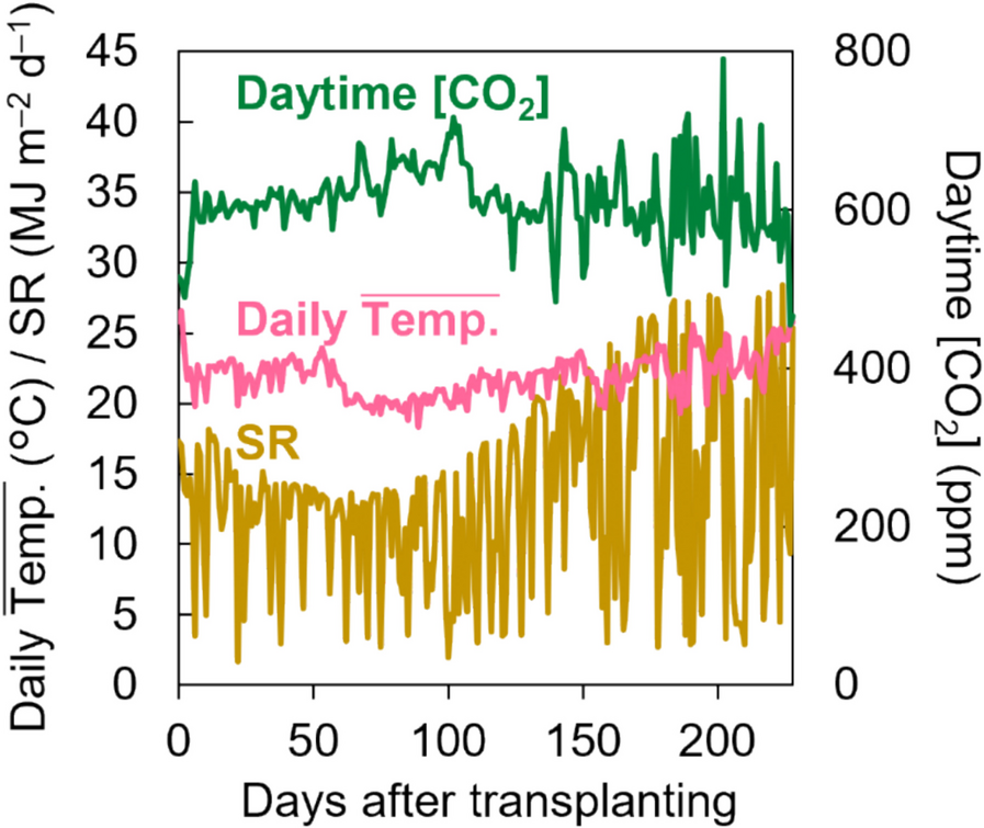
To demonstrate the potential effects of cultivar-dependent variation in shoot architecture on cucumber yield, we selected four commercially available Japanese cultivars (‘Josho’, ‘S-30’, ‘G-Flush’, and ‘Yusho’), which are recognized for their different levels of vigor. The experiment was conducted in 2021, with plants grown in a greenhouse under the conditions shown in Fig. 1. We assessed node numbers and found that ‘Josho’ had formed more nodes than all other cultivars by the end of cultivation period (Fig. 2A). Then, we analyzed changes in the NFR, calculated as the number of nodes formed per unit of daily average temperature, throughout the experiment (Fig. 2B). The NFR was higher in ‘Josho’ than in the other cultivars, particularly ‘S-30’ and ‘Yusho’. The mean NFRs were 2.2 × 10^–2 nodes °C^–1 day^–1 for ‘Josho’ and approximately 1.5 × 10^–2 nodes °C^–1 day^–1 for the other cultivars. A similar trend was observed in a separate short-term experiment conducted in a different greenhouse and year (Fig. S2), suggesting that the observed differences are cultivar-dependent rather than condition-dependent. We also noted cultivar-specific variation in the position of open female flowers along the stem. In ‘Josho’, open female flowers tended to appear at nodes farther from the shoot tip compared to the other cultivars (Fig. S3), implying more rapid stem growth. These findings indicate that the cultivars are distinguishable by their shoot architecture, particularly in terms of NFR and node number.

Comparison of fruit yield among cultivars

Final fresh yield was highest in ‘Josho’ (approximately 36.3 kg m^–2), consistent with its elevated NFR compared to the other cultivars (Fig. 2C). The number of harvested fruits followed a similar pattern: ‘Josho’ produced around 360 fruits per unit area, whereas the other cultivars yielded approximately 300 or fewer (Fig. 2D). Mean harvested fruit weight was around 100 g fruit^–1 (Fig. S4A). The ratio of aborted fruits, which were excluded from yield calculations, was higher in ‘Josho’ (approximately 7.4%) than in the others (1.0% or less, Fig. S4B). Female flowering rates were broadly similar across cultivars, although ‘G-Flush’ exhibited a slightly lower rate (Fig. S4C). These findings suggest that yield differences were primarily driven by variation in node formation, rather than by fruit abortion or female flowering frequency in the cultivars examined.

DM distribution

Next, we compared the cultivars in terms of how DM was partitioned to fruit. The experimental period was divided into five terms based on the timing of destructive measurements (term 1: 0–45 DAT; term 2: 45–66 DAT; term 3: 66–105 DAT; term 4: 105–142 DAT; term 5: 142–228 DAT), and DM partitioning was analyzed for each term. As shown in Fig. 3A, DM partitioning in ‘Josho’ during the first term was 0.15 g g^–1 and remained around 0.5 g g^–1 in later terms. In contrast, the other cultivars, particularly ‘Yusho’, showed higher early DM partitioning (approximately 0.2 g g^–1) but failed to maintain these levels beyond the third term. In the final term, DM partitioning in ‘S-30’, ‘G-Flush’, and ‘Yusho’ declined to approximately 0.4 g g^–1. As a result, the cumulative fruit dry yield relative to TDM in ‘Josho’ continued to increase, reaching 0.48 g g^–1 by the end of the experiment. In comparison, the other cultivars peaked at around 0.44 g g^–1 on 105 DAT and declined thereafter (Fig. S5A). Additionally, DM content per fruit was comparable across cultivars, confirming that fruit quality was consistent (Fig. S5B). Together, these results indicate that reduced node formation suppressed DM partitioning to fruit.

DM productivity

Although yield differences among the cultivars could be attributable to variation in both shoot architecture and DM productivity, this did not appear to be the case in the present experiment. TDM across the five experimental terms was largely comparable among cultivars, except during the third and final terms (Fig. 3A). Notably, ‘S-30’, but not ‘Josho’, tended to exhibit higher TDM. In the third and final terms, TDM in ‘S-30’ reached 417 and 1,484 g m^–2, respectively, while the values for ‘Josho’ were 348 and 1,431 g m^–2. ‘Yusho’ showed the lowest TDM in the final term (1,329 g m^–2). As LAI was maintained at approximately 2.4 m² m^–2 across all cultivars, cumulative IL was estimated to be similar among cultivars (around 650 MJ m^–2; Fig. S6). Consequently, LUE varied as shown in Figure S7, with ‘S-30’ exhibiting the highest LUE (4.26 g MJ^–1), followed by ‘G-Flush’ (4.08 g MJ^–1), ‘Josho’ (4.07 g MJ^–1), and ‘Yusho’ (3.86 g MJ^–1). Similar trends were observed in TDM at the end of the experiment (Fig. 3B). The discrepancies between yield and TDM or LUE suggest that DM productivity had only a marginal effect on yield differences among cultivars. Indeed, correlation analysis of the yield components revealed no significant relationship between yield and DM productivity. In contrast, a strong correlation was observed between node formation and fruit yield (Fig. 4). These findings demonstrate that cultivar-dependent shoot architecture can influence fruit yield independently of DM productivity in cucumber plants.

Transcriptomic diversity among cultivars

In cucumber plants, nodes are produced by the SAM while flowers develop from the leaf axil at each node [3], underscoring the importance of SAM activity for yield. Certain meristem identity-regulating genes determine whether the SAM exhibits determinate or indeterminate growth in Cucumis sativus [3]. These findings suggest genetic diversity among the shoot tips of the four cultivars. To explore this possibility, we performed mRNA-seq using RNA extracted from their shoot tips. We identified more than 500 differentially expressed genes (DEGs), assessed using the criteria |fold change|> 2 and false discovery rate (FDR) < 0.05, in pairwise comparisons between ‘Josho’ and the other cultivars (Figs. 5 and S8, and Dataset S1). We also examined the expression of genes previously reported to regulate SAM identity (Table S1), including PEBPs involved in floral meristem induction (CsFT, CsTFL1, CsTFL1d); subunits of protein complexes including CsFT or CsTFL1/CsTFL1d (CsNOT2a, CsFD, CsFDP, CsGF14-3, CsGF14-5); and transcription factors and their interactors involved in SAM maintenance and floral meristem differentiation (CsLFY, CsWUS, CsUFO, CsHAN1, CsHAN2, CsSTM, CsBP). We initially expected some of these genes to meet the criteria for differential expression, but none qualified as DEGs. However, CsTFL1 in ‘S-30’, CsGF14-3 and CsGF14-5 in ‘G-Flush’, and CsBP in all three cultivars showed modest reductions (approximately 30% on average) compared to ‘Josho’ (Dataset S2). To further investigate physiological differences, we conducted Gene Ontology (GO) enrichment analysis of DEGs common among ‘S-30’, ‘G-Flush’, and ‘Yusho’. We selected 42 downregulated and 16 upregulated genes and analyzed their enrichment in biological processes. Only one GO term was significantly enriched among upregulated genes, related to carbon fixation. This term included two DEGs: CsaV3_4G001210, which encodes a putative CP12 domain-containing protein, and CsaV3_6G048750, a putative RbcX homolog (Fig. S9A and Datasets S3 and S4). In contrast, downregulated DEGs were enriched for GO terms associated with heat response, cell division, and β-oxidation. These included putative condensin proteins (CsaV3_UNG044290, CsaV3_UNG075600, CsaV3_UNG088700, CsaV3_UNG225770), heat-shock proteins and co-chaperones (CsaV3_1G035820, CsaV3_1G035830, CsaV3_1G044020, CsaV3_3G006720, CsaV3_5G026520), a multiprotein bridging factor 1c (MBF1c) homolog (CsaV3_2G002310), an ankyrin repeat-containing protein (CsaV3_1G010260), and 3-hydroxyacyl-CoA dehydrogenase proteins (CsaV3_6G023960, CsaV3_6G024070, CsaV3_024110) (Fig. S9B and Datasets S3 and S4). These findings indicate that the shoot tips of the four cultivars differ at the transcriptional level, which may reflect genetic factors underlying the observed variation in NFR.

Experimental setup

The experimental setup included a (Delta.3) haptic robot (Force Dimension, Switzerland) placed on a desk next to a display monitor (Fig. 1). The device is capable of measuring positions and providing forces up to 20.0 N in the three translational directions (x, y, and z axes, Fig. 1). The device control was implemented in C++, operating at 4 kHz. Motion data was recorded at 1.67 kHz.

The pendulum game

The game, inspired by the work of [44] and created in Unity 3D (Unity Technologies, USA), consisted of controlling a virtual pendulum to hit moving targets approaching the participant. The pendulum consisted of a black ball (pivoting point) and a red ball (pendulum mass), with a rigid link connecting both balls, as shown in Figs. 1 and 2. The pendulum’s pivoting point could be moved horizontally and vertically (y and z axis in Fig. 2) by displacing the haptic device’s end-effector (black ball in Fig. 1 Right; 1:1 movement mapping). The pendulum could only swing in the vertical plane (y–z), and therefore, movements of the haptic device in the x-direction were not mapped to the pendulum.

The task consisted of hitting vertical targets with the pendulum mass. The targets were located on walls approaching the participants in the x direction, i.e., perpendicular to the screen plane. The walls were spaced by 1 m and their speed was set to 1 m/s. The targets could appear in three different positions: the center point of the wall or ± 0.12 m to the right/left. The target’s width was 0.02 m, and the pendulum ball and pivoting point diameter were set to 0.03 m.

By moving the pendulum pivoting point through the device end-effector, participants influenced the swing of the pendulum, which behaved according to the equation of motion of a simple pendulum:

where y and z are the horizontal and vertical coordinates of the robot end-effector position and (ddot{theta }) the angular acceleration of the pendulum’s internal degree of freedom (DoF). Since the internal DoF was located at the pendulum’s pivoting point, (theta ) was defined relative to the pendulum rod, as illustrated in Fig. 2. The robot’s coordinates were referenced with respect to its initial position after calibration, similar to the one shown in Fig. 1right. The pendulum mass was set to (m = 0.6) kg, the rod length to (l = 0.25) m, gravity to (g = 3.24) m/(s^2), and the constant (c = 3.00e^{-6}) N(cdot )s/rad. These parameters were adjusted and chosen in order to minimize passive stabilization of the pendulum and maintain task difficulty.

As the pendulum crossed a wall, a score based on the absolute distance of the pendulum’s mass to the center of the target in the y-direction (|Error|) was briefly displayed for 0.5 s to provide feedback regarding participants’ performance. The score ranged between 0 and 100 and was calculated as:

Each phase of the experiment was organized into wall sets, with 20 walls presented per set (see the Study protocol Section). A final score, based on the average of all 20 scores, was shown at the end of each set to inform participants of their overall performance in that set.

Haptic rendering and haptic guidance

To enhance the ecological validity of the task — ensuring the experimental conditions closely replicate real-world scenarios — we incorporated haptic rendering throughout the whole experiment, i.e., the provision of the forces originating from the pendulum dynamics on the device end-effector. Participants could feel the pendulum force dynamics ((F_{rod})), calculated as:

using the same constants as in Eq. (1).

Participants allocated to the Experimental group were also provided with haptic guidance during training to physically assist them in the target-hitting task. This was achieved by first calculating an optimal end-effector trajectory between the pendulum state at the moment of target wall collision and the target at the following wall, and then enforcing this trajectory using a Proportional-Derivative (PD) controller.

The optimal end-effector trajectory was calculated every time the pendulum hit a target wall using the ACADO toolkit [45]. The cost function included terms to maximize accuracy (i.e., minimize the distance between the pendulum ball and the next target’s centerline), maximize the pendulum stabilization (i.e., penalizing the velocity components of the pendulum ball), and minimize end-effector acceleration based on the current state of the pendulum, as described in the Appendix B.

The PD controller aimed to minimize the distance between the end-effector and the reference trajectory in the y-direction at each time point by applying a guiding force (F_{HG}) at the end-effector. We only provided guidance in the y-axis as it was sufficient to achieve the target-hitting tasks. By not guiding in the z-direction, we also reduced the potential masking effects of the guidance on the perception of the haptic rendering of the pendulum dynamics. The resulting equation for the PD controller is as follows:

where the y-axis error between the actual and the reference trajectory was denoted as e(t), and the proportional ((K_p)) and derivative ((K_d)) gains were set to 75.0 N/m and 15 N(cdot )s/m, respectively. The guiding force was added to the haptic rendering force ((F_{rod}) in Eq. (3)). The order of magnitude of the guidance force was around four times the haptic rendering.

Participants

Forty-two unimpaired participants performed the experiment. Data from two participants were excluded from further analysis. One participant exhibited errors three standard deviations higher than the average of all participants. We encountered a technical problem when recording the data of a second participant, leading to missing data within the dataset. Thus, 40 participants were included in the analysis (age = (27 pm 6,yrs); 19 identified as female, 21 identified as male; no participants identified as non-binary). The target sample size of approximately 40 participants was determined based on a power analysis, as detailed in Appendix A. Handedness was assessed using the Short-Form Edinburgh Handedness Inventory [46], resulting in 35 right-handed, four left-handed, and one ambidextrous participant. All participants signed the informed consent to participate in the study, which was approved by the TU Delft Human Research Ethics Committee (HREC).

Participants were allocated into two training groups: Control or Experimental. The Experimental group received haptic guidance during some parts of the training phase (see the Study protocol Section), while the Control group practiced without any physical assistance. To promote an even distribution between groups, we used an adaptive randomization method. We randomly allocated the first twenty participants into one of the two training groups and distributed new ones into each group based on their sex and results from the Locus of Control questionnaire (see the Outcome metrics Section), similar to [7]. The Locus of Control was employed as it directly relates to the perception of control, which aligned with the groups’ training conditions (guidance vs. no guidance).

Study protocol

The experiment was conducted in two locations: Delft University of Technology, Delft, the Netherlands, and Alten Netherlands B.V., Rotterdam, the Netherlands. The experimental setup and protocol were identical in both locations. Minor environmental differences (e.g., room layout, lighting) were not expected to systematically affect performance. The overview of the experimental protocol can be found in Fig. 3.

The experiment took place in two sessions on different days, with one to three days between sessions, following recommendations to evaluate motor learning [3]. At the beginning of the first session, participants were invited to sit at the set-up table. The chair height was adjusted based on personal preferences to ensure a comfortable arm movement within the robot’s workspace. The haptic device was placed at a reachable distance with a relaxed posture on the dominant hand’s side. The screen was placed on the opposite side of the device in front of the participant. Participants were informed about the goal of the pendulum task at the beginning of the first session. No extra information was given during the rest of the experiment.

The experiment began by inviting participants to fill out the first block of questionnaires, including demographic data collection and the questionnaires to quantify the personality traits (see the Outcome metrics Section). Participants were then invited to familiarize themselves with the haptic device and the virtual environment for 40 s. During this familiarization phase, they were asked to move the pendulum freely in the virtual environment without loading any target. They could observe the pendulum moving and feel the haptic rendering of the pendulum dynamics through the haptic device end-effector. Once the 40 s were over, participants were instructed again about the game goal: move the pendulum such that the red ball hits each wall as close as possible to the target’s center. They were then invited to play a first set of 20 targets.

Once the familiarization was completed, the main experiment began. Participants underwent three main phases during Session 1: baseline, training, and short-term retention. During these phases, participants performed one or three different tasks. The main task consisted of playing 20 targets in a specific order. Each time the main task was played, targets were set in the same sequence of positions, except during the training phase, in which some of the sets were mirrored (further explained later in this section). Participants also played two transfer tasks to asses the generalization of the acquired skill. Those tasks were similar to the main task but included slight design variations. In the position transfer task, the targets were randomly re-located (still appearing every 1 s) to introduce new movement sequences. During the dynamics transfer task, the target positions were kept the same as during the main task, but the pendulum dynamics were changed. While the appearance of the pendulum did not change, the pendulum rod length was reduced by 70% in Eq. (1) and (3). This variation affected the pendulum’s natural frequency, which increased from 0.573 Hz to 0.685 Hz. For both transfer tasks, the goal remained the same: Use the pendulum mass to hit each target.

The baseline included two sets of 20 targets for the main task. The game did not stop between sets within the same task, but there was an extended pause of three seconds in which no new targets were loaded. After the second set was finalized, participants completed a new set of questionnaires to assess motivation and agency. To keep our analysis focused on answering the listed hypotheses, the analysis of motivation and agency are out of the scope of this work. Participants were then asked to play the game two more times, for two sets of the position transfer task and two sets of the dynamics transfer task, with an on-demand break offered between the two tasks.

After the baseline trials were complete, participants began the training. They completed two rounds of 15 sets of the main task of 20 targets each. Participants had the opportunity to take a break between rounds. During training, the Experimental group received haptic guidance on top of the haptic rendering. However, to avoid participant reliance on the guidance, guidance was removed during the first set and once every five sets (“catch sets”). In addition, to avoid only learning the specific movement patterns and target positions, mirrored sets were interspersed within the non-catch sets for both groups. The position of the targets during these sets was mirrored with respect to the walls’ y-axis. The distribution of “catch sets” and mirrored sets can be found in Fig. 3. Participants were informed that they might or might not be assisted during training to promote active participation. The Control group only experienced the haptic rendering from the pendulum dynamics during training.

Immediately following the last training set, participants took a 10-minute break. During this time, they filled in a new set of questionnaires. The Experimental group was asked questions about their subjective experience with the robotic guidance, i.e., how disturbing, frustrating or restrictive it was perceived (see the Outcome metrics Section). Following the break, a washout set of the main task was conducted by both groups to mitigate any temporary effects from training with haptic guidance, e.g., “slacking” [47].

Right after the washout set, participants performed the short-term retention phase. The structure was similar to the baseline but without the questionnaire. Participants returned after one to three days to perform a long-term retention phase, which was structured identically to the baseline tests.

Outcome metrics

Personality traits questionnaires

Before the familiarization phase, participants completed a battery of questionnaires assessing the selected personality traits to study. These personality traits included the LOC scale [34], the Transform of Challenge and Transform of Boredom sub-scales from the Autotelic personality questionnaire [33], and the Achiever and Free Spirit sections of the Hexad Gaming style questionnaire [39]. All the questionnaires, except for the LOC, were formed by seven-point-based questions and normalized between 0 and 1 (low to high level of trait/characteristic). The LOC questionnaire was formed by 23 multiple-choice questions, and the overall score for the whole questionnaire ranged from 0 to 23. To improve interpretability and facilitate later modeling (see the Statistical analysis Section), this range was normalized from -1 to 1 to reflect the continuum between Internal LOC (-1) and External LOC (1), which are widely recognized classifications in literature and commonly used to interpret behavior. In addition, the LOC scores usually follow an approximate Gaussian distribution centered near zero. This makes this range statistically practical and close to the centered scale. Internal and external LOC differ in whether outcomes from an action are attributed to oneself or external circumstances, respectively. The employed questions for all the questionnaires can be found in the Appendix C.

Human-robot interaction experience questionnaire

Three questions were filled in by only the Experimental group after training. These questions related to frustration, disturbance, and restrictiveness perception during the training (see Appendix C). They were answered on a seven-point scale, which was then normalized between 0 and 1 (low to high).

Task performance: absolute error

To assess motor learning, the distance between the pendulum’s mass position and each target’s centerline at the time of pendulum-wall contact was calculated (|Error|), in meters. This was used as our performance metric and one value per wall was obtained.

Human-robot interaction: interaction force

To assess participants’ interaction with the haptic device, the human-robot interaction force was estimated. This estimate was computed using Reaction Torque Observers based on recorded motor currents and the robot dynamic model, as implemented in [44]. For the analysis, we used the average force per target in Newtons. We calculated this average force within the interval from consecutive midpoints between walls.

Statistical analysis

To evaluate the hypotheses outlined in the Introduction Section, we used Linear Mixed Models (LMMs). These models were fitted using the (texttt{lmer}) function from the (texttt{lmerTest}) package in (texttt{R}). Statistical significance was set at (p < 0.05), and p-values were adjusted for multiple comparisons using Bonferroni correction.

The employed LMMs were selected as outlined in Appendix D. We group them throughout the current section depending on the hypotheses they are tailored to evaluate. Table 1 summarizes the variables that can be included in the models. Task performance (|Error|) and human-robot interaction force (|IntForce|) metrics were analyzed as dependent variables depending on the model. Logarithmic transformations were applied to correct skewed distributions and achieve normality requirements.

Models to infer motor learning (M1.1 and M1.2)

To evaluate the impact of personality traits and the training condition on motor learning outcomes across different experimental phases (related to hypotheses H1 and H2) we employed two models, one for each dependent variable. These models include independent variables regarding the training group, the task type, the stage, and the personality traits (see description in Table 1). Given the extensive number of variables and potential interactions, a stepwise comparison between models of different complexity was performed using the Akaike Information Criterion (AIC) and Bayesian Information Criterion (BIC) to prevent overfitting and ensure stability (see Appendix D).

For the performance metric (|Error|), the following model (M1.1) with the smallest AIC and BIC was chosen:

In this equation, the normalized and centered results from the Transform of Challenge ((TC_c)) and Locus of Control (LOC_c) were included as traits of interest, as others did not show statistical significance during model selection. Therefore, the hypothesis related to the Achiever gaming style (H1.3) is not supported by the data. A nested random effect for wall index (wIndex : NewWalls) was adjusted to account for changes in wall positioning during the position-based transfer task.

A similar model (M1.2) was developed for the interaction force metric. Notably, this model included an additional interaction term, (Group times LOC_c times Stage). When compared with other configurations, the model with this extra interaction led to a lower AIC and slightly increased BIC (see Appendix D). In view of these competing results, previous literature was used to guide the choice. This extra relationship was considered of interest as LOC was found to correlate to the interaction force metric during the training phase when the haptic guidance was active (see [43]). The final model has the form:

Note that while this model does not include the Free Spirit gaming style, results from an alternative model (see Appendixes D and E) suggest a potential relationship between this trait and interaction force outcomes, which can be considered of interest for hypothesis H1.4. Yet, fully evaluating this effect would require studying the model complexity beyond the current study’s scope, complicating the understanding of the results. As such, we leave a thorough investigation of H1.4 for future work.    

Human-robot interaction perception model (M2)

To investigate whether subjective perceptions of human-robot interaction (HRI) influenced task performance (H3), we employed the following model:

where the HRIQuestion represents the normalized and centered response to each of the specific HRI perception questions. The normalized and centered version of four of the traits were considered of interest for this model, i.e., the Achiever ((AC_c)) and Free Spirit ((FS_c)) gaming styles, Transform of Challenge ((TC_c)), and Locus of Control ((LOC_c)). All the phases were included in this dataset (baseline, training, short- and long-term retention) while the transfer tasks were excluded as HRI questions were asked exclusively after the training phase, which did not include the transfer tasks.

Unlock the Editor’s Digest for free

Roula Khalaf, Editor of the FT, selects her favourite stories in this weekly newsletter.

Anthropic plans to invest $50bn in building artificial intelligence infrastructure in the US over the coming years, as the start-up races to secure new computing power.

The Claude chatbot maker on Wednesday said it would develop new data centres in New York and Texas with UK-based cloud computing start-up Fluidstack. The sites will bolster Anthropic’s research and development as well as providing power for its existing AI tools.

“We’re getting closer to AI that can accelerate scientific discovery and help solve complex problems in ways that weren’t possible before. Realising that potential requires infrastructure that can support continued development at the frontier,” said Dario Amodei, chief executive and co-founder of Anthropic.

The investment follows a flurry of deals by Anthropic’s chief rival OpenAI to secure chips and computing capacity from Nvidia, AMD, Broadcom, Oracle and Google, estimated to be worth about $1.5tn.

The circular arrangements between companies that act as suppliers, investors and customers of each other, combined with booming AI valuations, have added to concerns about a bubble in the sector.

Anthropic has also moved to boost its computing power this year. Last month, the four-year-old start-up signed a deal to secure access to 1mn Google Cloud chips to train and run its AI models.

The San Francisco-based group also has a partnership with Amazon, which is the start-up’s “primary” cloud provider and a large investor. It has invested $8bn in Anthropic and is building a 2.2GW data-centre cluster in New Carlisle, Indiana, to help train its AI models.

Its latest agreement will involve it partnering with Fluidstack, a small start-up that this year signed a deal with the French government to build a major computing cluster in France. Anthropic said it chose the company for its “exceptional agility”.

“We’re proud to partner with frontier AI leaders like Anthropic to accelerate and deploy the infrastructure necessary to realise their vision,” said Gary Wu, co-founder and CEO of Fluidstack.

Anthropic, which was recently valued at $183bn post-money, was founded by a group of former OpenAI employees. While OpenAI has focused largely on its consumer product ChatGPT, Anthropic has targeted enterprise customers.

The group’s run-rate revenue — a projection of annual revenue based on recent performance which is favoured by start-ups — shot from $1bn at the start of the year to $7bn last month. In September the company raised $13bn from investors including Iconiq Capital and Lightspeed Venture Partners.

Introduction

On behalf of the New York Fed, let me welcome you all to this year’s U.S. Treasury Market Conference. Many thanks to the distinguished speakers and panelists for joining us here, and to the event organizers for putting together today’s outstanding agenda. I’m looking forward to a valuable and productive conversation.

This gathering is a recurring calendar item every fall. But the topics that we discuss each year do not stand alone. Think of it as leveling up in a video game—which is one of my favorite pastimes by the way, or dare I say, “present times”. At each conference, we advance our understanding of the Treasury market to the next level. And in the genre of gaming, this game is multiplayer. It’s remarkable to think about what we’ve accomplished in this decade-long enterprise of interagency collaboration. This work continues to be imperative, so we must keep playing. I mean that in the working sense, of course.

Before I keep going, I must give the standard Fed disclaimer that the views I express today are mine alone and do not necessarily reflect those of the Federal Open Market Committee (FOMC) or others in the Federal Reserve System.

Three Levels of Play

The remarks that I’ve given at past conferences have focused on taking stock of the Treasury market and sharing updates on our collective efforts.¹ My comments today will be a retrospective into the events, developments, and lessons learned over the past seven years. I will then explain how all of that has shaped the FOMC’s thinking around monetary policy implementation and the design of our ample reserves implementation framework. I’ll also bring you up to speed with regard to where the Federal Reserve stands on its balance sheet strategy.

So, let’s return to the video game analogy and start at level one—the episode of volatility known as the “flash rally” of 2014. That period of market stress served as a sharp reminder that financial markets are not static: they evolve in response to changes in technology, regulation, business models, and with the addition of new players and participants.

That initial level made it clear that safeguards and systems must evolve so that these markets can continue to function well in every circumstance and under any condition. So, from there, we jumped to the next level. And that’s the imperative of market resiliency. We learned the importance of creating a system that can better withstand the unforeseeable and the unpredictable. Because when the unforeseeable and unpredictable did happen, as we saw in the “dash-for-cash” in 2020, it resulted in significant stresses in the Treasury market and related markets that threatened to spread to broader financial conditions.

This leads me to level three. A resilient financial system is critically important for monetary policy. Because monetary policy influences the economy by affecting financial market conditions, its effectiveness relies on well-functioning markets, with the Treasury market at the heart of it all.

Good news—we’ve unlocked the next level of my remarks. And that is an explanation of the FOMC’s approach to monetary policy implementation to support effective interest rate control and smooth functioning of these core markets.

Framing the Frameworks

We’ve established that monetary policy implementation frameworks are critically important to the conduct of monetary policy.²

In supplying reserves to the banking system, the Federal Reserve has multiple goals that frequently involve trade-offs.³ First and foremost, it targets a level of the policy interest rate and aims to minimize the variability of the policy rate around that target. In addition, it has objectives related to supporting financial stability and the smooth functioning of financial markets.

The core of any operational framework is the supply of reserves, which can range from a low level, or “scarce,” to “ample” and “abundant.” The “price” of reserves is the spread between the market interest rate and the rate earned for holding reserves at the central bank. When reserves are scarce, the slope of the demand curve for reserves is steep. A small change in the quantity of reserves results in a meaningful change in the spread. When reserves are ample, the demand curve flattens but still slopes downward, so that small changes in the quantity of reserves have modest effects on the spread. And when reserves are abundant, the demand curve is essentially flat.

A central bank has two sets of tools it can use to supply reserves. First, it chooses an ex ante aggregate level of reserves to supply to the banking system. Second, it may make available lending facilities to the banking system that offer loans to financial institutions at an interest rate determined by the central bank. If the ex ante supply of reserves is sufficiently low, the additional demand will be met by the lending facilities. Note that both tools are a means to supply reserves: In the first, the supply is set in advance, while with the latter, it adjusts endogenously to market conditions.

It is worth emphasizing that the two tools can be mutually reinforcing in achieving desired outcomes. For example, lending facilities limit upward movements in interest rates on days of high demand, thereby reducing the ex ante supply of reserves needed to control short-term rates.⁴

Federal Reserve: Ample Reserves and Tools

The Fed’s operational framework has evolved over time, reflecting its experience with large balance sheets since the global financial crisis.⁵ In January 2019, when the decline in the Fed’s asset holdings implied that the quantity of reserves would soon fall below an “abundant” level, the FOMC formally adopted an ample reserves strategy.⁶

The FOMC has defined this framework as one in which “control over the level of the federal funds rate and other short-term interest rates is exercised primarily through the setting of the Federal Reserve’s administered rates, and in which active management of the supply of reserves is not required.”⁷ Accordingly, the ex ante supply of reserves is chosen to be sufficiently large to meet the demand for reserves on most days.

One important tool the FOMC has established to ensure interest rate control is the overnight reverse repo facility (ON RRP), which, alongside the interest paid on reserve balances (IORB), helps set a floor for the federal funds rate. Through the ON RRP, eligible counterparties “lend” to the Federal Reserve at the rate set by the FOMC, currently at the bottom of the target range for the federal funds rate. Usage of the ON RRP adjusts automatically to market conditions, rising and falling with supply and demand, which is particularly important in a dynamic market.

The ON RRP has proven to be a very effective and flexible tool to support interest rate control to the downside. When Federal Reserve asset holdings push reserves above ample, the ON RRP relaxes the tight relationship between balance sheet size and reserves and acts as a safety valve in supporting smooth transmission of monetary policy to markets. As the size of the balance sheet falls, market rates rise above the rate offered at the ON RRP and, as a result, usage of the ON RRP declines to very low levels. The dynamic usage of the ONRRP is seen in Figure 1, which shows average monthly usage of the ON RRP from 2016 through October of this year. The ON RRP was used extensively when it was economically sensible for the Fed’s counterparties to do so. By contrast, it has very limited usage when repo rates are well above the ON RRP rate, as is the case today.

In 2021, the Federal Reserve introduced the Standing Repo Facility (SRF), which nicely complements the ON RRP by providing interest rate control to the upside.⁸ The SRF rate is set at the top of the FOMC’s target range for the federal funds rate. This combination of an ample supply of reserves and an SRF rate at the top of the target range reduces the day-to-day reliance on the facility except during periods of significant upward pressure on rates resulting from strong liquidity demand or market stress.

By ensuring that adequate liquidity will be available in a wide variety of circumstances, the SRF plays a critical role in capping temporary upward pressure on rates and assures markets of effective interest rate control and smooth market functioning. It is best thought of as a way of making sure that the overall market has adequate liquidity consistent with the FOMC’s desired level of interest rates. In that regard, it differs from other lending facilities—such as the discount window—that aim to provide individual banks with liquidity when the need arises.

The SRF has been effective as reserves have moved from abundant toward ample. Over the past two months, SRF usage has risen from essentially zero to having greater frequency and higher volume of take-up, especially on days of temporary repo market pressures, as shown in Figure 2. Like the ON RRP facility, the SRF’s effectiveness relies on market participants availing themselves of the SRF based on market conditions, free of worries about stigma or other impediments. I fully expect that the SRF will continue to be actively used in this way and contain upward pressures on money market rates.

Federal Reserve: The Way Forward

At the onset of the pandemic, the Fed, along with central banks around the world, responded quickly to restore market functioning,⁹ causing reserves to rise well above ample, as they did in many jurisdictions.

In June of 2022, the Fed began the process of reducing the size of its balance sheet to transition toward an ample level of reserves.¹⁰ The FOMC said it intended to stop balance sheet runoff when it deemed reserves were somewhat above ample, and then allow reserves to decline further as other liabilities, such as currency, grow.

The process has worked according to plan. The Fed’s securities holdings have shrunk from a peak of about $8-1/2 trillion in 2022 to $6-1/4 trillion today. At its meeting in October, the FOMC decided it would conclude the reduction of its aggregate securities holdings on December 1.¹¹ This decision was based on clear market-based signs that we had met the test of reserves being somewhat above ample.¹² In particular, repo rates have increased relative to administered rates and have exhibited more volatility on certain days. Accordingly, we have been seeing more frequent use of the SRF. And the effective federal funds rate has increased somewhat relative to the IORB after years of that spread being at a stable level. These developments were expected as the supply of reserves closed in on ample.¹³

Looking forward, the next step in our balance sheet strategy will be to assess when the level of reserves has reached ample. It will then be time to begin the process of gradual purchases of assets that will maintain an ample level of reserves as the Fed’s other liabilities grow and underlying demand for reserves increases over time. Such reserve management purchases will represent the natural next stage of the implementation of the FOMC’s ample reserves strategy and in no way represent a change in the underlying stance of monetary policy.

Determining when we are at ample reserves is an inexact science. I am closely monitoring a variety of market indicators related to the fed funds market, repo market, and payments to help assess the state of reserve demand conditions. Based on recent sustained repo market pressures and other growing signs of reserves moving from abundant to ample, I expect that it will not be long before we reach ample reserves.

Conclusion

With that, we’ve arrived at the endgame of my remarks. We’ve learned a lot over the past decade. The FOMC’s monetary policy implementation framework is designed to support an adequate supply of liquidity under a wide range of circumstances. The combination of an ample supply of reserves and the Standing Repo Facility enables the Committee to maintain strong interest rate control and flexibility regarding changes in the size of its balance sheet. This operational framework has proven to be highly effective—and continues to work as designed.

Figures

How many pounds of rice do you think you eat in a year? According to USA Rice, the average American enjoys 27 pounds annually — equivalent to the weight of a case of bottled water. In fact, rice isn’t just a mainstay in pantries, it’s a staple for more than half the world, and a vital source of income for 19%¹ of the world’s population.

With extreme weather events—such as droughts, floods, pests, and diseases—threatening rice yields and demand for rice in the United States continuing to rise, it is crucial for industry leaders like Mars to advance supply chain resiliency strategies to secure the future of rice.

Rising to the Challenge: How Mars is Supporting Rice Farming Resilience
The Arkansas Delta is a region in the eastern part of Arkansas that stretches along the Mississippi River and is one of the most productive agricultural areas in the country. This area accounts for 49.3% of total U.S. rice production and 49.9% of the total acres planted in 2024². Today, its once-fertile fields are grappling with droughts, saltwater from rising sea levels and floods, among other challenges. These challenges all point to an urgent need for innovation to secure and maintain this essential crop’s environment — one grain at a time.

As the manufacturer of iconic brands like Ben’s Original™— one of the world’s most recognized rice brands — as well as Tasty Bite® and Seeds of Change™, Mars, the maker of more than 40 U.S. food, snacking and pet brands, deeply understands the role rice plays in kitchens across the U.S. and around the world. Rice is more than just a staple ingredient; it’s a cornerstone of culture and nourishment for more than four billion people worldwide. That’s why our role goes far beyond simply selling products — it’s about honoring rice’s global significance and supporting the communities, farmers and families who depend on it.

“As a leader in the rice industry, we recognize our opportunity to help farmers across our value chain address environmental challenges that threaten their livelihoods,” said Dave Dusangh, President Mars Food & Nutrition, North America. “By collaborating closely with our partner farmers, we are working to build a more sustainable, resilient and innovative rice supply chain that benefits both people and the planet.”

Innovating for a Water-Smart Future
We’re using our longstanding expertise and global resources to help farmers adopt and scale advanced agricultural techniques that conserve water while reducing greenhouse gas emissions.

Conventional rice cultivation often relies on continuously flooded fields, which is water intensive and restricts oxygen in the soil and creates conditions for methane-producing bacteria — leading to greenhouse gas emissions. Mars is helping farmers adopt innovative water management techniques and technologies that improve water efficiency, strengthen climate resilience, and cut emissions. A few of these examples include:

• Alternate wetting and drying (AWD): A water management technique that allows rice fields to alternate between periods of flooding and drying, rather than maintaining continuous flooding throughout the growing season. This approach has been shown to reduce the amount of water used by up to 30% and reduce the amount of GHG emissions produced by over 40%³ each growing season.
• Multiple inlet rice irrigation (MIRI): This system optimizes how water is delivered using multiple inlets in pipes placed across a field. This distributes water more efficiently, cutting down on water usage, and reducing emissions.
• Row rice, or furrow irrigation: A method that bypasses the need to flood fields, while improving ease of crop rotation. Using this technique, water is applied in rows rather than flooding across the entire section of the field.
• Zero-grade fields are precision-leveled to ensure a flat surface with no slope, allowing water to flow evenly across the field and eliminating the need for internal levees or side inlets. This minimizes the need for intensive tilling, further improving efficiency and enabling farmers to save up to 37%⁴ more water each growing season compared to traditional contoured or leveed fields.

While these are promising solutions, shifting away from traditional methods can be challenging. The cost of new systems, concern about potential yield loss and difficulty of changing longstanding habits all make adoption a challenge for many farmers. Mars is supporting farmers by paying premiums on top of the commodity price to incentivize the adoption of new practices, as well as sharing data so Mars can measure the environmental benefits of these practices. This data sharing has helped show farmers in the Mars rice supply chain that embracing these practices hasn’t negatively impacted their crop yields. In fact, research has shown that using zero-grade fields with the AWD irrigation method reduces water usage by 65%⁵ while still providing the same crop yields.

“The role Mars plays in helping us adopt climate-smart agriculture practices is critical because it gives us an incentive to go out there and try something new,” says Terry Gray, an Arkansas rice farmer in the Mars Food & Nutrition rice supply chain. “We’re trying out these practices to grow the same yields with less strain on the land — and the results are showing it’s better for the environment all around.”

Partnering to Protect Farmers and the Planet
“The challenges faced by rice farmers today demand bold leadership, and partners like Mars are vital in driving meaningful change,” said Peter Bachmann, President and CEO, USA Rice. “By leveraging its resources, expertise and scale, Mars is helping farmers adopt climate-smart agriculture practices that not only sustain their livelihoods but also safeguard the environment.”

At Mars, mutuality is one of our core guiding principles. Collaboration with partners throughout our supply chain is essential to how we’re working to shape a more secure future for farmers, communities and the planet. Our approach to rice farming reflects this value, as we address challenges and build the future we envision together, every step of the way.

Through a steadfast commitment to our Sustainable in a Generation plan, Mars is championing impactful innovation that strengthens U.S. rice farming, setting an example across global food systems in an ever-evolving world.
 

---

1. Rice – Rice Sector at a Glance | Economic Research Service. n.d. https://www.ers.usda.gov/topics/crops/rice/rice-sector-at-a-glance

2. Handbook, IPM, AND-STaR | Arkansas Cooperative Extension Service https://www.uaex.uada.edu/farm-ranch/crops-commercial-horticulture/rice/

3. Mars & Riceland Sustainable Rice Program (Arva Intelligence)

4. Massey et al. 2022, Direct Comparisons of four rice irrigation systems on a commercial rice farm, Agricultural Water Management, Vol 266, 31 May 2022 https://www.sciencedirect.com/science/article/abs/pii/S0378377422001536

5. Mars & Riceland Sustainable Rice Program (Arva Intelligence)