…
Category: 7. Science
-
3D morphology of the Cambrian bivalved arthropod Sunella informs about head segmentation, arthrodization, and arthropodization
Budd, G. E. & Telford, M. J. The origin and evolution of arthropods. Nature 457, 812–817 (2009).
Edgecombe, G. D. & Legg, D. A. Origins and early evolution of arthropods. Palaeontology 57,…
Continue Reading
-
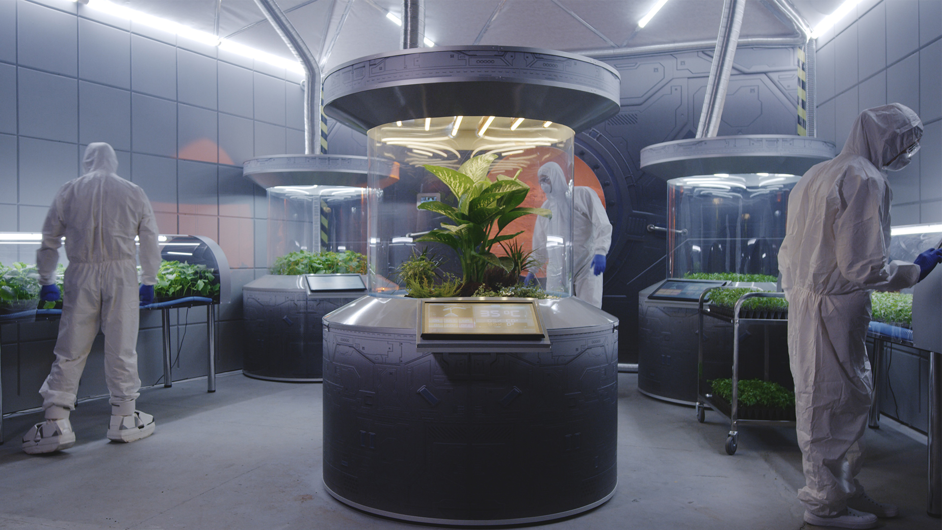
Cyanobacteria have the potential to turn Martian soil fertile
Imagine landing on Mars and growing your lunch—not with supplies from Earth, but using dust, air, and microbes already there. This idea has long sounded like science fiction, mainly because Mars lacks one critical ingredient, fertile soil. Its…
Continue Reading
-
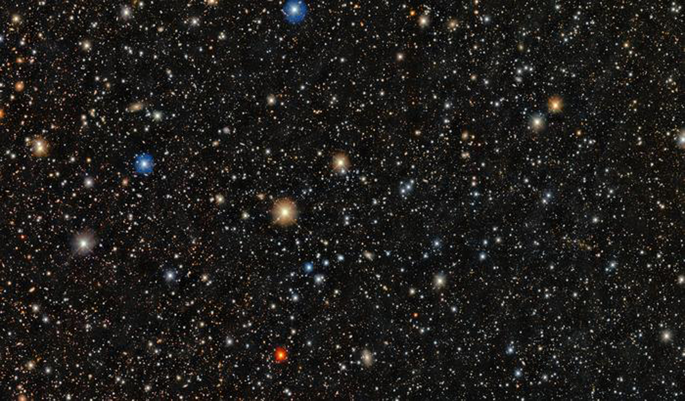
Ancient star reveals clues to the Milky Way’s outer halo origin
Researchers have identified an ancient star in a tiny satellite galaxy that preserves the clearest chemical record yet of the universe’s first stars.
That record points to a quieter kind of stellar explosion and links a long-standing mystery in…
Continue Reading
-
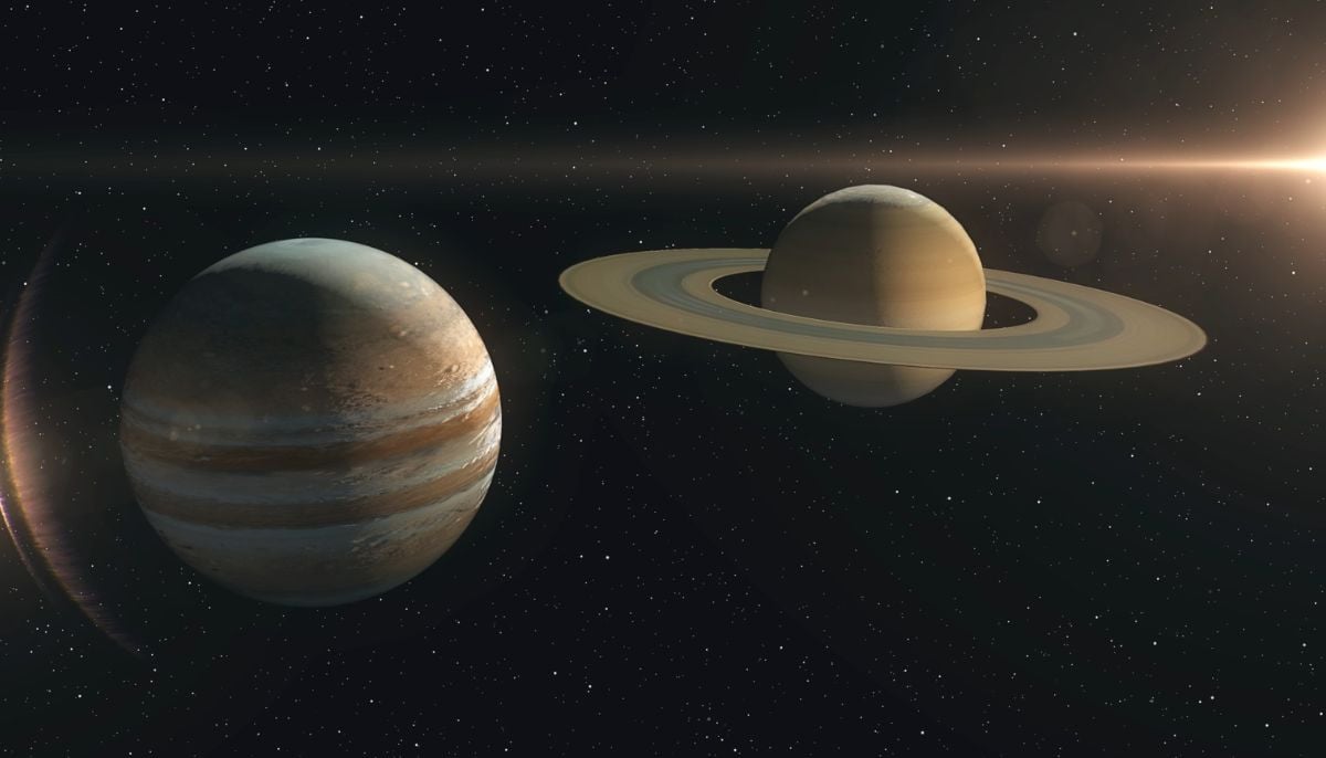
Scientists discover more moons orbiting Jupiter, Saturn
Most people do not understand that the solar system contains more objects than they…
Continue Reading
-
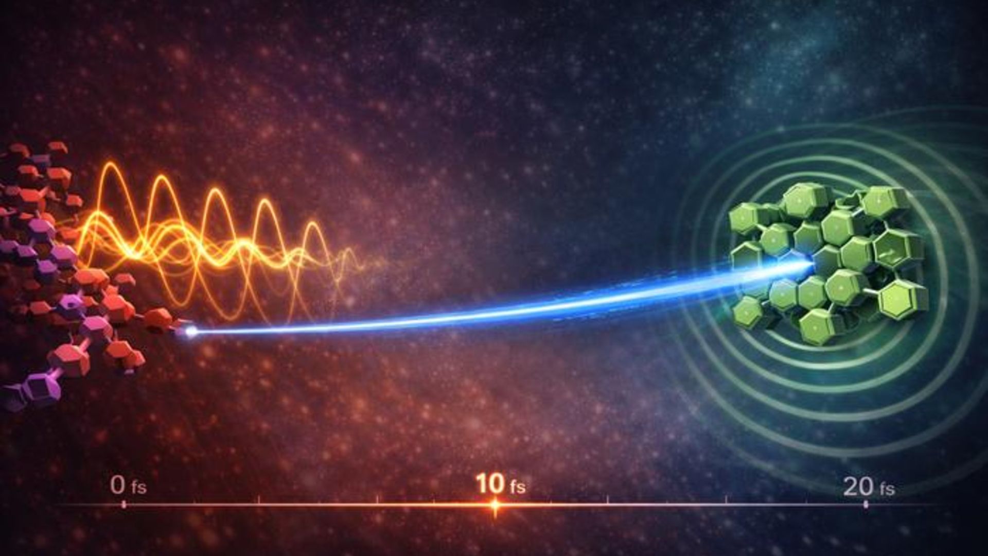
Physicists create electron ‘catapult’ that moves particles through solar cells at record speed
Molecular vibrations can “catapult” electrons across solar materials in quadrillionths of a second — much faster than previously thought, a new study shows.
The findings could help scientists find more efficient ways to convert solar…
Continue Reading
-
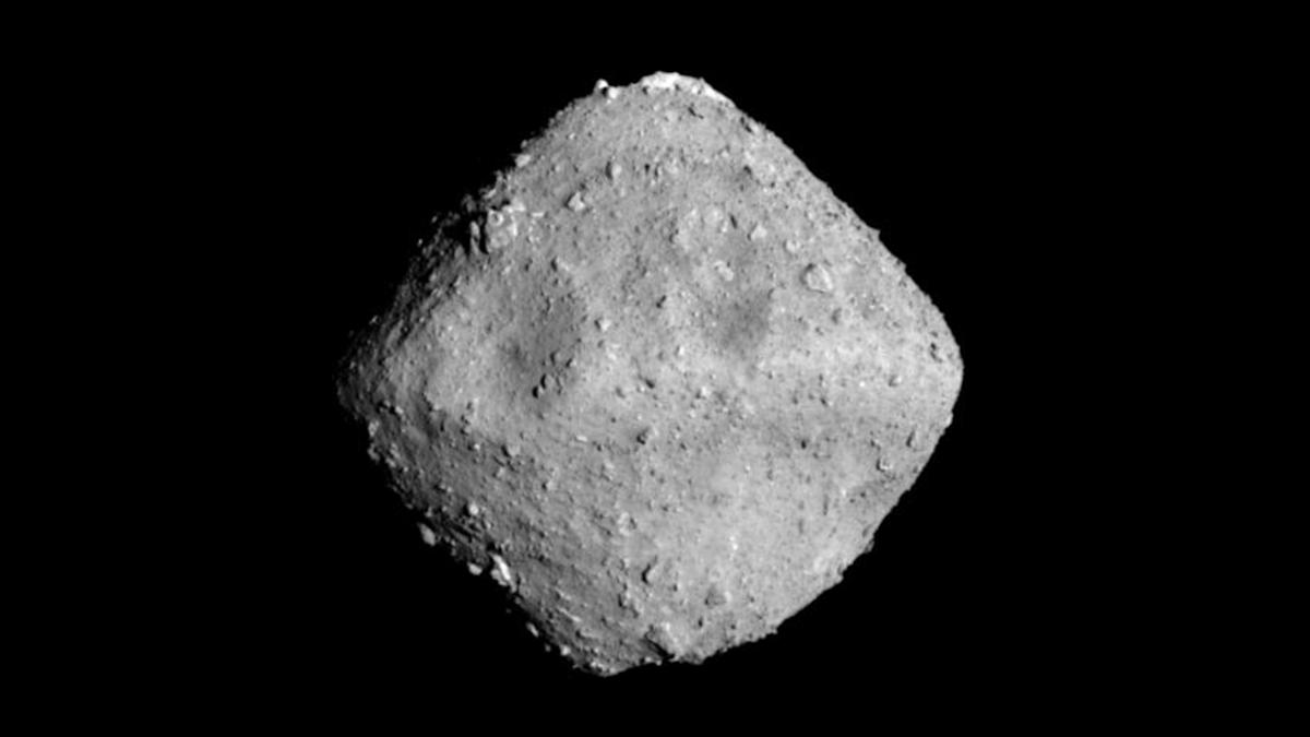
DNA building blocks on asteroid Ryugu, bacteria that eat plastic waste, and more science news
Remember when Japan sent a spacecraft to an asteroid 180 million miles away to scoop some dirt off the surface? Six years on from its arrival to Earth, that sample has yielded some insights about what may have seeded life on our planet. Read on…
Continue Reading
-

The Longest Animal On Earth Has No Brain, No Bones And 1,200 Stingers — A Biologist Explains
In 1865, a dead jellyfish washed onto a Massachusetts beach. When scientists measured it, they discovered that its bell measured 2.1 meters (7 feet) across, making it wider than most doorways. What was more shocking were its tentacles: they…
Continue Reading